（转）A Beginner's Guide To Understanding Convolutional Neural Networks

Adit Deshpande

CS Undergrad at UCLA ('19)

Blog About

A Beginner's Guide To Understanding Convolutional Neural Networks

Introduction

Convolutional neural networks. Sounds like a weird combination of biology and math with a little CS sprinkled in, but these networks have been some of the most influential innovations in the field of computer vision. 2012 was the first year that neural nets grew to prominence as Alex Krizhevsky used them to win that year’s ImageNet competition (basically, the annual Olympics of computer vision), dropping the classification error record from 26% to 15%, an astounding improvement at the time.Ever since then, a host of companies have been using deep learning at the core of their services. Facebook uses neural nets for their automatic tagging algorithms, Google for their photo search, Amazon for their product recommendations, Pinterest for their home feed personalization, and Instagram for their search infrastructure.

However, the classic, and arguably most popular, use case of these networks is for image processing. Within image processing, let’s take a look at how to use these CNNs for image classification.

The Problem Space

Image classification is the task of taking an input image and outputting a class (a cat, dog, etc) or a probability of classes that best describes the image. For humans, this task of recognition is one of the first skills we learn from the moment we are born and is one that comes naturally and effortlessly as adults. Without even thinking twice, we’re able to quickly and seamlessly identify the environment we are in as well as the objects that surround us. When we see an image or just when we look at the world around us, most of the time we are able to immediately characterize the scene and give each object a label, all without even consciously noticing. These skills of being able to quickly recognize patterns, generalize from prior knowledge, and adapt to different image environments are ones that we do not share with our fellow machines.

Inputs and Outputs

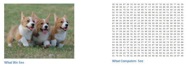
When a computer sees an image (takes an image as input), it will see an array of pixel values. Depending on the resolution and size of the image, it will see a 32 x 32 x 3 array of numbers (The 3 refers to RGB values). Just to drive home the point, let's say we have a color image in JPG form and its size is 480 x 480. The representative array will be 480 x 480 x 3. Each of these numbers is given a value from 0 to 255 which describes the pixel intensity at that point. These numbers, while meaningless to us when we perform image classification, are the only inputs available to the computer.  The idea is that you give the computer this array of numbers and it will output numbers that describe the probability of the image being a certain class (.80 for cat, .15 for dog, .05 for bird, etc).

What We Want the Computer to Do

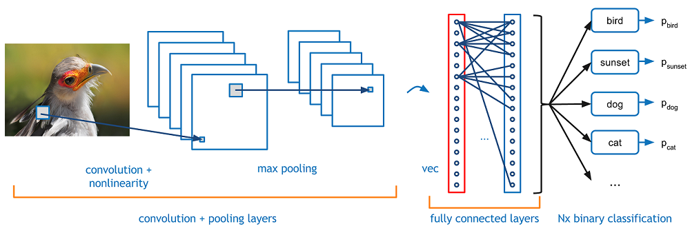
Now that we know the problem as well as the inputs and outputs, let’s think about how to approach this. What we want the computer to do is to be able to differentiate between all the images it’s given and figure out the unique features that make a dog a dog or that make a cat a cat. This is the process that goes on in our minds subconsciously as well. When we look at a picture of a dog, we can classify it as such if the picture has identifiable features such as paws or 4 legs. In a similar way, the computer is able perform image classification by looking for low level features such as edges and curves, and then building up to more abstract concepts through a series of convolutional layers. This is a general overview of what a CNN does. Let’s get into the specifics.

Biological Connection

But first, a little background. When you first heard of the term convolutional neural networks, you may have thought of something related to neuroscience or biology, and you would be right. Sort of. CNNs do take a biological inspiration from the visual cortex. The visual cortex has small regions of cells that are sensitive to specific regions of the visual field. This idea was expanded upon by a fascinating experiment by Hubel and Wiesel in 1962 (Video) where they showed that some individual neuronal cells in the brain responded (or fired) only in the presence of edges of a certain orientation. For example, some neurons fired when exposed to vertical edges and some when shown horizontal or diagonal edges. Hubel and Wiesel found out that all of these neurons were organized in a columnar architecture and that together, they were able to produce visual perception. This idea of specialized components inside of a system having specific tasks (the neuronal cells in the visual cortex looking for specific characteristics) is one that machines use as well, and is the basis behind CNNs.

Structure

Back to the specifics. A more detailed overview of what CNNs do would be that you take the image, pass it through a series of convolutional, nonlinear, pooling (downsampling), and fully connected layers, and get an output. As we said earlier, the output can be a single class or a probability of classes that best describes the image. Now, the hard part is understanding what each of these layers do. So let’s get into the most important one.

First Layer – Math Part

The first layer in a CNN is always a Convolutional Layer. First thing to make sure you remember is what the input to this conv (I’ll be using that abbreviation a lot) layer is. Like we mentioned before, the input is a 32 x 32 x 3 array of pixel values. Now, the best way to explain a conv layer is to imagine a flashlight that is shining over the top left of the image. Let’s say that the light this flashlight shines covers a 5 x 5 area. And now, let’s imagine this flashlight sliding across all the areas of the input image. In machine learning terms, this flashlight is called a filter(or sometimes referred to as a neuron or a kernel) and the region that it is shining over is called the receptive field. Now this filter is also an array of numbers (the numbers are called weights orparameters). A very important note is that the depth of this filter has to be the same as the depth of the input (this makes sure that the math works out), so the dimensions of this filter is 5 x 5 x 3. Now, let’s take the first position the filter is in for example.  It would be the top left corner. As the filter is sliding, or convolving, around the input image, it is multiplying the values in the filter with the original pixel values of the image (aka computing element wise multiplications). These multiplications are all summed up (mathematically speaking, this would be 75 multiplications in total). So now you have a single number. Remember, this number is just representative of when the filter is at the top left of the image. Now, we repeat this process for every location on the input volume. (Next step would be moving the filter to the right by 1 unit, then right again by 1, and so on). Every unique location on the input volume produces a number. After sliding the filter over all the locations, you will find out that what you’re left with is a 28 x 28 x 1 array of numbers, which we call an activation map or feature map. The reason you get a 28 x 28 array is that there are 784 different locations that a 5 x 5 filter can fit on a 32 x 32 input image. These 784 numbers are mapped to a 28 x 28 array.

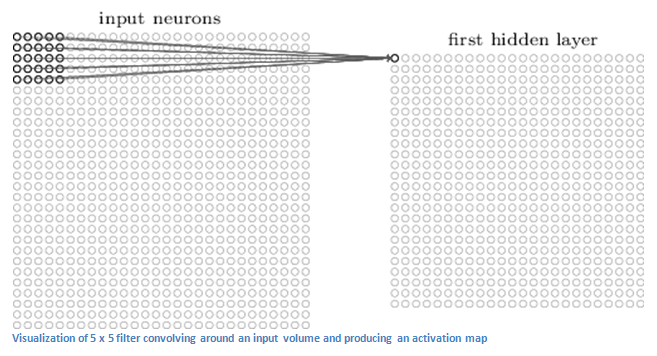
(Quick Note: Some of the images, including the one above, I used came from this terrific book, "Neural Networks and Deep Learning" by Michael Nielsen. Strongly recommend.)

Let’s say now we use two 5 x 5 x 3 filters instead of one. Then our output volume would be 28 x 28 x 2. By using more filters, we are able to preserve the spatial dimensions better. Mathematically, this is what’s going on in a convolutional layer.

First Layer – High Level Perspective

However, let’s talk about what this convolution is actually doing from a high level. Each of these filters can be thought of as feature identifiers. When I say features, I’m talking about things like straight edges, simple colors, and curves. Think about the simplest characteristics that all images have in common with each other. Let’s say our first filter is 7 x 7 x 3 and is going to be a curve detector. (In this section, let’s ignore the fact that the filter is 3 units deep and only consider the top depth slice of the filter and the image, for simplicity.)As a curve detector, the filter will have a pixel structure in which there will be higher numerical values along the area that is a shape of a curve (Remember, these filters that we’re talking about as just numbers!).

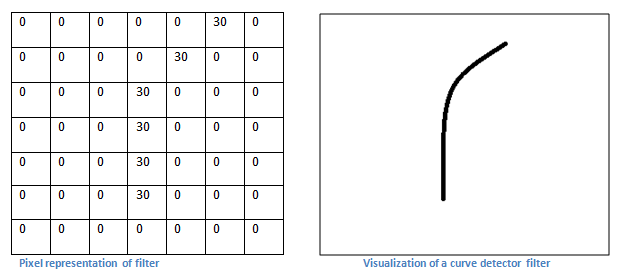
Now, let’s go back to visualizing this mathematically. When we have this filter at the top left corner of the input volume, it is computing multiplications between the filter and pixel values at that region. Now let’s take an example of an image that we want to classify, and let’s put our filter at the top left corner.

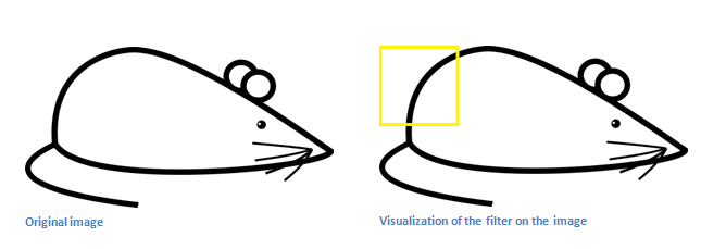
Remember, what we have to do is multiply the values in the filter with the original pixel values of the image.

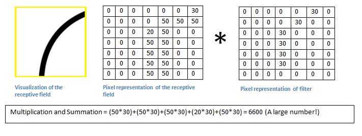
Basically, in the input image, if there is a shape that generally resembles the curve that this filter is representing, then all of the multiplications summed together will result in a large value! Now let’s see what happens when we move our filter.

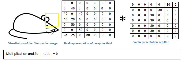
The value is much lower! This is because there wasn’t anything in the image section that responded to the curve detector filter. Remember, the output of this conv layer is an activation map. So, in the simple case of a one filter convolution (and if that filter is a curve detector), the activation map will show the areas in which there at mostly likely to be curves in the picture. In this example, the top left value of our 28 x 28 x 1 activation map will be 6600. This high value means that it is likely that there is some sort of curve in the input volume that caused the filter to activate. The top right value in our activation map will be 0 because there wasn’t anything in the input volume that caused the filter to activate (or more simply said, there wasn’t a curve in that region of the original image). Remember, this is just for one filter. This is just a filter that is going to detect lines that curve outward and to the right. We can have other filters for lines that curve to the left or for straight edges. The more filters, the greater the depth of the activation map, and the more information we have about the input volume.

Disclaimer: The filter I described in this section was simplistic for the main purpose of describing the math that goes on during a convolution. In the picture below, you’ll see some examples of actual visualizations of the filters of the first conv layer of a trained network. Nonetheless, the main argument remains the same. The filters on the first layer convolve around the input image and “activate” (or compute high values) when the specific feature it is looking for is in the input volume.

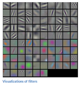
(Quick Note: The above image came from Stanford's CS 231N course taught by Andrej Karpathy and Justin Johnson. Recommend for anyone looking for a deeper understanding of CNNs.)

Going Deeper Through the Network

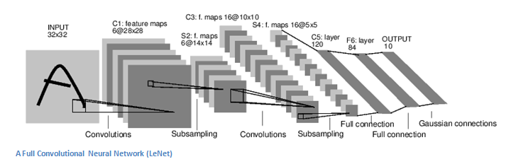
Now in a traditional convolutional neural network architecture, there are other layers that are interspersed between these conv layers. I’d strongly encourage those interested to read up on them and understand their function and effects, but in a general sense, they provide nonlinearities and preservation of dimension that help to improve the robustness of the network and control overfitting. A classic CNN architecture would look like this.

The last layer, however, is an important one and one that we will go into later on. Let’s just take a step back and review what we’ve learned so far. We talked about what the filters in the first conv layer are designed to detect. They detect low level features such as edges and curves. As one would imagine, in order to predict whether an image is a type of object, we need the network to be able to recognize higher level features such as hands or paws or ears. So let’s think about what the output of the network is after the first conv layer. It would be a 28 x 28 x 3 volume (assuming we use three 5 x 5 x 3 filters).  When we go through another conv layer, the output of the first conv layer becomes the input of the 2nd conv layer.  Now, this is a little bit harder to visualize. When we were talking about the first layer, the input was just the original image. However, when we’re talking about the 2nd conv layer, the input is the activation map(s) that result from the first layer. So each layer of the input is basically describing the locations in the original image for where certain low level features appear. Now when you apply a set of filters on top of that (pass it through the 2nd conv layer), the output will be activations that represent higher level features. Types of these features could be semicircles (combination of a curve and straight edge) or squares (combination of several straight edges). As you go through the network and go through more conv layers, you get activation maps that represent more and more complex features. By the end of the network, you may have some filters that activate when there is handwriting in the image, filters that activate when they see pink objects, etc. If you want more information about visualizing filters in ConvNets, Matt Zeiler and Rob Fergus had an excellentresearch paper discussing the topic. Jason Yosinski also has a video on YouTube that provides a great visual representation. Another interesting thing to note is that as you go deeper into the network, the filters begin to have a larger and larger receptive field, which means that they are able to consider information from a larger area of the original input volume (another way of putting it is that they are more responsive to a larger region of pixel space).

Fully Connected Layer

Now that we can detect these high level features, the icing on the cake is attaching a fully connected layer to the end of the network. This layer basically takes an input volume (whatever the output is of the conv or ReLU or pool layer preceding it) and outputs an N dimensional vector where N is the number of classes that the program has to choose from. For example, if you wanted a digit classification program, N would be 10 since there are 10 digits. Each number in this N dimensional vector represents the probability of a certain class. For example, if the resulting vector for a digit classification program is [0 .1 .1 .75 0 0 0 0 0 .05], then this represents a 10% probability that the image is a 1, a 10% probability that the image is a 2, a 75% probability that the image is a 3, and a 5% probability that the image is a 9 (Side note: There are other ways that you can represent the output, but I am just showing the softmax approach). The way this fully connected layer works is that it looks at the output of the previous layer (which as we remember should represent the activation maps of high level features) and determines which features most correlate to a particular class. For example, if the program is predicting that some image is a dog, it will have high values in the activation maps that represent high level features like a paw or 4 legs, etc. Similarly, if the program is predicting that some image is a bird, it will have high values in the activation maps that represent high level features like wings or a beak, etc. Basically, a FC layer looks at what high level features most strongly correlate to a particular class and has particular weights so that when you compute the products between the weights and the previous layer, you get the correct probabilities for the different classes.

Training (AKA:What Makes this Stuff Work)

Now, this is the one aspect of neural networks that I purposely haven’t mentioned yet and it is probably the most important part. There may be a lot of questions you had while reading. How do the filters in the first conv layer know to look for edges and curves? How does the fully connected layer know what activation maps to look at? How do the filters in each layer know what values to have? The way the computer is able to adjust its filter values (or weights) is through a training process called backpropagation.

Before we get into backpropagation, we must first take a step back and talk about what a neural network needs in order to work. At the moment we all were born, our minds were fresh. We didn’t know what a cat or dog or bird was. In a similar sort of way, before the CNN starts, the weights or filter values are randomized. The filters don’t know to look for edges and curves. The filters in the higher layers don’t know to look for paws and beaks. As we grew older however, our parents and teachers showed us different pictures and images and gave us a corresponding label. This idea of being given an image and a label is the training process that CNNs go through. Before getting too into it, let’s just say that we have a training set that has thousands of images of dogs, cats, and birds and each of the images has a label of what animal that picture is. Back to backprop.

So backpropagation can be separated into 4 distinct sections, the forward pass, the loss function, the backward pass, and the weight update. During the forward pass, you take a training image which as we remember is a 32 x 32 x 3 array of numbers and pass it through the whole network. On our first training example, since all of the weights or filter values were randomly initialized, the output will probably be something like [.1 .1 .1 .1 .1 .1 .1 .1 .1 .1], basically an output that doesn’t give preference to any number in particular. The network, with its current weights, isn’t able to look for those low level features or thus isn’t able to make any reasonable conclusion about what the classification might be. This goes to the loss function part of backpropagation. Remember that what we are using right now is training data. This data has both an image and a label. Let’s say for example that the first training image inputted was a 3. The label for the image would be [0 0 0 1 0 0 0 0 0 0]. A loss function can be defined in many different ways but a common one is MSE (mean squared error), which is ½ times (actual - predicted) squared.

Let’s say the variable L is equal to that value. As you can imagine, the loss will be extremely high for the first couple of training images. Now, let’s just think about this intuitively. We want to get to a point where the predicted label (output of the ConvNet) is the same as the training label (This means that our network got its prediction right).In order to get there, we want to minimize the amount of loss we have. Visualizing this as just an optimization problem in calculus, we want to find out which inputs (weights in our case) most directly contributed to the loss (or error) of the network.

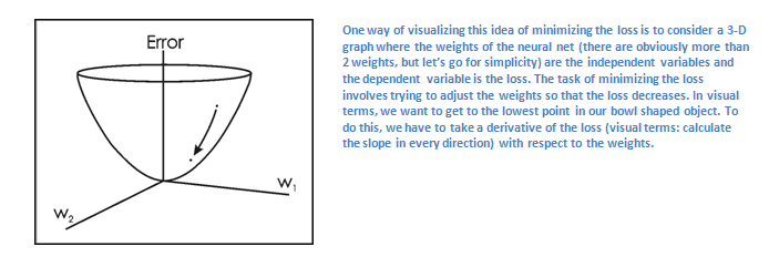
This is the mathematical equivalent of a dL/dW where W are the weights at a particular layer. Now, what we want to do is perform a backward pass through the network, which is determining which weights contributed most to the loss and finding ways to adjust them so that the loss decreases. Once we compute this derivative, we then go to the last step which is the weight update. This is where we take all the weights of the filters and update them so that they change in the direction of the gradient.

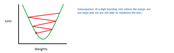
The learning rate is a parameter that is chosen by the programmer. A high learning rate means that bigger steps are taken in the weight updates and thus, it may take less time for the model to converge on an optimal set of weights. However, a learning rate that is too high could result in jumps that are too large and not precise enough to reach the optimal point.

The process of forward pass, loss function, backward pass, and parameter update is generally called one epoch. The program will repeat this process for a fixed number of epochs for each training image. Once you finish the parameter update on the last training example, hopefully the network should be trained well enough so that the weights of the layers are tuned correctly.

Testing

Finally, to see whether or not our CNN works, we have a different set of images and labels (can’t double dip between training and test!) and pass the images through the CNN. We compare the outputs to the ground truth and see if our network works!

How Companies Use CNNs

Data, data, data. The companies that have lots of this magic 4 letter word are the ones that have an inherent advantage over the rest of the competition. The more training data that you can give to a network, the more training iterations you can make, the more weight updates you can make, and the better tuned to the network is when it goes to production. Facebook (and Instagram) can use all the photos of the billion users it currently has, Pinterest can use information of the 50 billion pins that are on its site, Google can use search data, and Amazon can use data from the millions of products that are bought every day. And now you know the magic behind how they use it.

Disclaimer  

While this post should be a good start to understanding CNNs, it is by no means a comprehensive overview. Things not discussed in this post include the nonlinear and pooling layers as well as hyperparameters of the network such as filter sizes, stride, and padding. Topics like network architecture, batch normalization, vanishing gradients, dropout, initialization techniques, non-convex optimization,biases, choices of loss functions, data augmentation,regularization methods, computational considerations, modifications of backpropagation, and more were also not discussed (yet ).

Link to Part 2

Dueces.

Sources

Written on July 20, 2016