10分钟学习pandas
10 Minutes to pandas
This is a short introduction to pandas, geared mainly for new users. You can see more complex recipes in the Cookbook
Customarily, we import as follows:
In [1]: import pandas as pd

In [2]: import numpy as np

In [3]: import matplotlib.pyplot as plt
Object Creation
See the Data Structure Intro section
Creating a Series by passing a list of values, letting pandas create a default integer index:
In [4]: s = pd.Series([1,3,5,np.nan,6,8])

In [5]: s

Out[5]:

0    1.0

1    3.0

2    5.0

3    NaN

4    6.0

5    8.0

dtype: float64
Creating a DataFrame by passing a numpy array, with a datetime index and labeled columns:
In [6]: dates = pd.date_range('20130101', periods=6)

In [7]: dates

Out[7]:

DatetimeIndex(['2013-01-01', '2013-01-02', '2013-01-03', '2013-01-04',

               '2013-01-05', '2013-01-06'],

              dtype='datetime64[ns]', freq='D')

In [8]: df = pd.DataFrame(np.random.randn(6,4), index=dates, columns=list('ABCD'))

In [9]: df

Out[9]:

                   A         B         C         D

2013-01-01  0.469112 -0.282863 -1.509059 -1.135632

2013-01-02  1.212112 -0.173215  0.119209 -1.044236

2013-01-03 -0.861849 -2.104569 -0.494929  1.071804

2013-01-04  0.721555 -0.706771 -1.039575  0.271860

2013-01-05 -0.424972  0.567020  0.276232 -1.087401

2013-01-06 -0.673690  0.113648 -1.478427  0.524988
Creating a DataFrame by passing a dict of objects that can be converted to series-like.
In [10]: df2 = pd.DataFrame({ 'A' : 1.,

   ....:                      'B' : pd.Timestamp('20130102'),

   ....:                      'C' : pd.Series(1,index=list(range(4)),dtype='float32'),

   ....:                      'D' : np.array([3] * 4,dtype='int32'),

   ....:                      'E' : pd.Categorical(["test","train","test","train"]),

   ....:                      'F' : 'foo' })

   ....:

In [11]: df2

Out[11]:

     A          B    C  D      E    F

0  1.0 2013-01-02  1.0  3   test  foo

1  1.0 2013-01-02  1.0  3  train  foo

2  1.0 2013-01-02  1.0  3   test  foo

3  1.0 2013-01-02  1.0  3  train  foo
Having specific dtypes
In [12]: df2.dtypes

Out[12]:

A           float64

B    datetime64[ns]

C           float32

D             int32

E          category

F            object

dtype: object
If you’re using IPython, tab completion for column names (as well as public attributes) is automatically enabled. Here’s a subset of the attributes that will be completed:
In [13]: df2.<TAB>

df2.A                  df2.boxplot

df2.abs                df2.C

df2.add                df2.clip

df2.add_prefix         df2.clip_lower

df2.add_suffix         df2.clip_upper

df2.align              df2.columns

df2.all                df2.combine

df2.any                df2.combineAdd

df2.append             df2.combine_first

df2.apply              df2.combineMult

df2.applymap           df2.compound

df2.as_blocks          df2.consolidate

df2.asfreq             df2.convert_objects

df2.as_matrix          df2.copy

df2.astype             df2.corr

df2.at                 df2.corrwith

df2.at_time            df2.count

df2.axes               df2.cov

df2.B                  df2.cummax

df2.between_time       df2.cummin

df2.bfill              df2.cumprod

df2.blocks             df2.cumsum

df2.bool               df2.D
As you can see, the columns A, B, C, and D are automatically tab completed. E is there as well; the rest of the attributes have been truncated for brevity.
Viewing Data
See the Basics section
See the top & bottom rows of the frame
In [14]: df.head()

Out[14]:

                   A         B         C         D

2013-01-01  0.469112 -0.282863 -1.509059 -1.135632

2013-01-02  1.212112 -0.173215  0.119209 -1.044236

2013-01-03 -0.861849 -2.104569 -0.494929  1.071804

2013-01-04  0.721555 -0.706771 -1.039575  0.271860

2013-01-05 -0.424972  0.567020  0.276232 -1.087401

In [15]: df.tail(3)

Out[15]:

                   A         B         C         D

2013-01-04  0.721555 -0.706771 -1.039575  0.271860

2013-01-05 -0.424972  0.567020  0.276232 -1.087401

2013-01-06 -0.673690  0.113648 -1.478427  0.524988
Display the index, columns, and the underlying numpy data
In [16]: df.index

Out[16]:

DatetimeIndex(['2013-01-01', '2013-01-02', '2013-01-03', '2013-01-04',

               '2013-01-05', '2013-01-06'],

              dtype='datetime64[ns]', freq='D')

In [17]: df.columns

Out[17]: Index([u'A', u'B', u'C', u'D'], dtype='object')

In [18]: df.values

Out[18]:

array([[ 0.4691, -0.2829, -1.5091, -1.1356],

       [ 1.2121, -0.1732,  0.1192, -1.0442],

       [-0.8618, -2.1046, -0.4949,  1.0718],

       [ 0.7216, -0.7068, -1.0396,  0.2719],

       [-0.425 ,  0.567 ,  0.2762, -1.0874],

       [-0.6737,  0.1136, -1.4784,  0.525 ]])
Describe shows a quick statistic summary of your data
In [19]: df.describe()

Out[19]:

              A         B         C         D

count  6.000000  6.000000  6.000000  6.000000

mean   0.073711 -0.431125 -0.687758 -0.233103

std    0.843157  0.922818  0.779887  0.973118

min   -0.861849 -2.104569 -1.509059 -1.135632

25%   -0.611510 -0.600794 -1.368714 -1.076610

50%    0.022070 -0.228039 -0.767252 -0.386188

75%    0.658444  0.041933 -0.034326  0.461706

max    1.212112  0.567020  0.276232  1.071804
Transposing your data
In [20]: df.T

Out[20]:

   2013-01-01  2013-01-02  2013-01-03  2013-01-04  2013-01-05  2013-01-06

A    0.469112    1.212112   -0.861849    0.721555   -0.424972   -0.673690

B   -0.282863   -0.173215   -2.104569   -0.706771    0.567020    0.113648

C   -1.509059    0.119209   -0.494929   -1.039575    0.276232   -1.478427

D   -1.135632   -1.044236    1.071804    0.271860   -1.087401    0.524988
Sorting by an axis
In [21]: df.sort_index(axis=1, ascending=False)

Out[21]:

                   D         C         B         A

2013-01-01 -1.135632 -1.509059 -0.282863  0.469112

2013-01-02 -1.044236  0.119209 -0.173215  1.212112

2013-01-03  1.071804 -0.494929 -2.104569 -0.861849

2013-01-04  0.271860 -1.039575 -0.706771  0.721555

2013-01-05 -1.087401  0.276232  0.567020 -0.424972

2013-01-06  0.524988 -1.478427  0.113648 -0.673690
Sorting by values
In [22]: df.sort_values(by='B')

Out[22]:

                   A         B         C         D

2013-01-03 -0.861849 -2.104569 -0.494929  1.071804

2013-01-04  0.721555 -0.706771 -1.039575  0.271860

2013-01-01  0.469112 -0.282863 -1.509059 -1.135632

2013-01-02  1.212112 -0.173215  0.119209 -1.044236

2013-01-06 -0.673690  0.113648 -1.478427  0.524988

2013-01-05 -0.424972  0.567020  0.276232 -1.087401
Selection
Note
While standard Python / Numpy expressions for selecting and setting are intuitive and come in handy for interactive work, for production code, we recommend the optimized pandas data access methods, .at, .iat, .loc, .iloc and .ix.
See the indexing documentation Indexing and Selecting Data and MultiIndex / Advanced Indexing
Getting
Selecting a single column, which yields a Series, equivalent to df.A
In [23]: df['A']

Out[23]:

2013-01-01    0.469112

2013-01-02    1.212112

2013-01-03   -0.861849

2013-01-04    0.721555

2013-01-05   -0.424972

2013-01-06   -0.673690

Freq: D, Name: A, dtype: float64
Selecting via [], which slices the rows.
In [24]: df[0:3]

Out[24]:

                   A         B         C         D

2013-01-01  0.469112 -0.282863 -1.509059 -1.135632

2013-01-02  1.212112 -0.173215  0.119209 -1.044236

2013-01-03 -0.861849 -2.104569 -0.494929  1.071804

In [25]: df['20130102':'20130104']

Out[25]:

                   A         B         C         D

2013-01-02  1.212112 -0.173215  0.119209 -1.044236

2013-01-03 -0.861849 -2.104569 -0.494929  1.071804

2013-01-04  0.721555 -0.706771 -1.039575  0.271860
Selection by Label
See more in Selection by Label
For getting a cross section using a label
In [26]: df.loc[dates[0]]

Out[26]:

A    0.469112

B   -0.282863

C   -1.509059

D   -1.135632

Name: 2013-01-01 00:00:00, dtype: float64
Selecting on a multi-axis by label
In [27]: df.loc[:,['A','B']]

Out[27]:

                   A         B

2013-01-01  0.469112 -0.282863

2013-01-02  1.212112 -0.173215

2013-01-03 -0.861849 -2.104569

2013-01-04  0.721555 -0.706771

2013-01-05 -0.424972  0.567020

2013-01-06 -0.673690  0.113648
Showing label slicing, both endpoints are included
In [28]: df.loc['20130102':'20130104',['A','B']]

Out[28]:

                   A         B

2013-01-02  1.212112 -0.173215

2013-01-03 -0.861849 -2.104569

2013-01-04  0.721555 -0.706771
Reduction in the dimensions of the returned object
In [29]: df.loc['20130102',['A','B']]

Out[29]:

A    1.212112

B   -0.173215

Name: 2013-01-02 00:00:00, dtype: float64
For getting a scalar value
In [30]: df.loc[dates[0],'A']

Out[30]: 0.46911229990718628
For getting fast access to a scalar (equiv to the prior method)
In [31]: df.at[dates[0],'A']

Out[31]: 0.46911229990718628
Selection by Position
See more in Selection by Position
Select via the position of the passed integers
In [32]: df.iloc[3]

Out[32]:

A    0.721555

B   -0.706771

C   -1.039575

D    0.271860

Name: 2013-01-04 00:00:00, dtype: float64
By integer slices, acting similar to numpy/python
In [33]: df.iloc[3:5,0:2]

Out[33]:

                   A         B

2013-01-04  0.721555 -0.706771

2013-01-05 -0.424972  0.567020
By lists of integer position locations, similar to the numpy/python style
In [34]: df.iloc[[1,2,4],[0,2]]

Out[34]:

                   A         C

2013-01-02  1.212112  0.119209

2013-01-03 -0.861849 -0.494929

2013-01-05 -0.424972  0.276232
For slicing rows explicitly
In [35]: df.iloc[1:3,:]

Out[35]:

                   A         B         C         D

2013-01-02  1.212112 -0.173215  0.119209 -1.044236

2013-01-03 -0.861849 -2.104569 -0.494929  1.071804
For slicing columns explicitly
In [36]: df.iloc[:,1:3]

Out[36]:

                   B         C

2013-01-01 -0.282863 -1.509059

2013-01-02 -0.173215  0.119209

2013-01-03 -2.104569 -0.494929

2013-01-04 -0.706771 -1.039575

2013-01-05  0.567020  0.276232

2013-01-06  0.113648 -1.478427
For getting a value explicitly
In [37]: df.iloc[1,1]

Out[37]: -0.17321464905330858
For getting fast access to a scalar (equiv to the prior method)
In [38]: df.iat[1,1]

Out[38]: -0.17321464905330858
Boolean Indexing
Using a single column’s values to select data.
In [39]: df[df.A > 0]

Out[39]:

                   A         B         C         D

2013-01-01  0.469112 -0.282863 -1.509059 -1.135632

2013-01-02  1.212112 -0.173215  0.119209 -1.044236

2013-01-04  0.721555 -0.706771 -1.039575  0.271860
A where operation for getting.
In [40]: df[df > 0]

Out[40]:

                   A         B         C         D

2013-01-01  0.469112       NaN       NaN       NaN

2013-01-02  1.212112       NaN  0.119209       NaN

2013-01-03       NaN       NaN       NaN  1.071804

2013-01-04  0.721555       NaN       NaN  0.271860

2013-01-05       NaN  0.567020  0.276232       NaN

2013-01-06       NaN  0.113648       NaN  0.524988
Using the isin() method for filtering:
In [41]: df2 = df.copy()

In [42]: df2['E'] = ['one', 'one','two','three','four','three']

In [43]: df2

Out[43]:

                   A         B         C         D      E

2013-01-01  0.469112 -0.282863 -1.509059 -1.135632    one

2013-01-02  1.212112 -0.173215  0.119209 -1.044236    one

2013-01-03 -0.861849 -2.104569 -0.494929  1.071804    two

2013-01-04  0.721555 -0.706771 -1.039575  0.271860  three

2013-01-05 -0.424972  0.567020  0.276232 -1.087401   four

2013-01-06 -0.673690  0.113648 -1.478427  0.524988  three

In [44]: df2[df2['E'].isin(['two','four'])]

Out[44]:

                   A         B         C         D     E

2013-01-03 -0.861849 -2.104569 -0.494929  1.071804   two

2013-01-05 -0.424972  0.567020  0.276232 -1.087401  four
Setting
Setting a new column automatically aligns the data by the indexes
In [45]: s1 = pd.Series([1,2,3,4,5,6], index=pd.date_range('20130102', periods=6))

In [46]: s1

Out[46]:

2013-01-02    1

2013-01-03    2

2013-01-04    3

2013-01-05    4

2013-01-06    5

2013-01-07    6

Freq: D, dtype: int64

In [47]: df['F'] = s1
Setting values by label
In [48]: df.at[dates[0],'A'] = 0
Setting values by position
In [49]: df.iat[0,1] = 0
Setting by assigning with a numpy array
In [50]: df.loc[:,'D'] = np.array([5] * len(df))
The result of the prior setting operations
In [51]: df

Out[51]:

                   A         B         C  D    F

2013-01-01  0.000000  0.000000 -1.509059  5  NaN

2013-01-02  1.212112 -0.173215  0.119209  5  1.0

2013-01-03 -0.861849 -2.104569 -0.494929  5  2.0

2013-01-04  0.721555 -0.706771 -1.039575  5  3.0

2013-01-05 -0.424972  0.567020  0.276232  5  4.0

2013-01-06 -0.673690  0.113648 -1.478427  5  5.0
A where operation with setting.
In [52]: df2 = df.copy()

In [53]: df2[df2 > 0] = -df2

In [54]: df2

Out[54]:

                   A         B         C  D    F

2013-01-01  0.000000  0.000000 -1.509059 -5  NaN

2013-01-02 -1.212112 -0.173215 -0.119209 -5 -1.0

2013-01-03 -0.861849 -2.104569 -0.494929 -5 -2.0

2013-01-04 -0.721555 -0.706771 -1.039575 -5 -3.0

2013-01-05 -0.424972 -0.567020 -0.276232 -5 -4.0

2013-01-06 -0.673690 -0.113648 -1.478427 -5 -5.0
Missing Data
pandas primarily uses the value np.nan to represent missing data. It is by default not included in computations. See the Missing Data section
Reindexing allows you to change/add/delete the index on a specified axis. This returns a copy of the data.
In [55]: df1 = df.reindex(index=dates[0:4], columns=list(df.columns) + ['E'])

In [56]: df1.loc[dates[0]:dates[1],'E'] = 1

In [57]: df1

Out[57]:

                   A         B         C  D    F    E

2013-01-01  0.000000  0.000000 -1.509059  5  NaN  1.0

2013-01-02  1.212112 -0.173215  0.119209  5  1.0  1.0

2013-01-03 -0.861849 -2.104569 -0.494929  5  2.0  NaN

2013-01-04  0.721555 -0.706771 -1.039575  5  3.0  NaN
To drop any rows that have missing data.
In [58]: df1.dropna(how='any')

Out[58]:

                   A         B         C  D    F    E

2013-01-02  1.212112 -0.173215  0.119209  5  1.0  1.0
Filling missing data
In [59]: df1.fillna(value=5)

Out[59]:

                   A         B         C  D    F    E

2013-01-01  0.000000  0.000000 -1.509059  5  5.0  1.0

2013-01-02  1.212112 -0.173215  0.119209  5  1.0  1.0

2013-01-03 -0.861849 -2.104569 -0.494929  5  2.0  5.0

2013-01-04  0.721555 -0.706771 -1.039575  5  3.0  5.0
To get the boolean mask where values are nan
In [60]: pd.isnull(df1)

Out[60]:

                A      B      C      D      F      E

2013-01-01  False  False  False  False   True  False

2013-01-02  False  False  False  False  False  False

2013-01-03  False  False  False  False  False   True

2013-01-04  False  False  False  False  False   True
Operations
See the Basic section on Binary Ops
Stats
Operations in general exclude missing data.
Performing a descriptive statistic
In [61]: df.mean()

Out[61]:

A   -0.004474

B   -0.383981

C   -0.687758

D    5.000000

F    3.000000

dtype: float64
Same operation on the other axis
In [62]: df.mean(1)

Out[62]:

2013-01-01    0.872735

2013-01-02    1.431621

2013-01-03    0.707731

2013-01-04    1.395042

2013-01-05    1.883656

2013-01-06    1.592306

Freq: D, dtype: float64
Operating with objects that have different dimensionality and need alignment. In addition, pandas automatically broadcasts along the specified dimension.
In [63]: s = pd.Series([1,3,5,np.nan,6,8], index=dates).shift(2)

In [64]: s

Out[64]:

2013-01-01    NaN

2013-01-02    NaN

2013-01-03    1.0

2013-01-04    3.0

2013-01-05    5.0

2013-01-06    NaN

Freq: D, dtype: float64

In [65]: df.sub(s, axis='index')

Out[65]:

                   A         B         C    D    F

2013-01-01       NaN       NaN       NaN  NaN  NaN

2013-01-02       NaN       NaN       NaN  NaN  NaN

2013-01-03 -1.861849 -3.104569 -1.494929  4.0  1.0

2013-01-04 -2.278445 -3.706771 -4.039575  2.0  0.0

2013-01-05 -5.424972 -4.432980 -4.723768  0.0 -1.0

2013-01-06       NaN       NaN       NaN  NaN  NaN
Apply
Applying functions to the data
In [66]: df.apply(np.cumsum)

Out[66]:

                   A         B         C   D     F

2013-01-01  0.000000  0.000000 -1.509059   5   NaN

2013-01-02  1.212112 -0.173215 -1.389850  10   1.0

2013-01-03  0.350263 -2.277784 -1.884779  15   3.0

2013-01-04  1.071818 -2.984555 -2.924354  20   6.0

2013-01-05  0.646846 -2.417535 -2.648122  25  10.0

2013-01-06 -0.026844 -2.303886 -4.126549  30  15.0

In [67]: df.apply(lambda x: x.max() - x.min())

Out[67]:

A    2.073961

B    2.671590

C    1.785291

D    0.000000

F    4.000000

dtype: float64
Histogramming
See more at Histogramming and Discretization
In [68]: s = pd.Series(np.random.randint(0, 7, size=10))

In [69]: s

Out[69]:

0    4

1    2

2    1

3    2

4    6

5    4

6    4

7    6

8    4

9    4

dtype: int64

In [70]: s.value_counts()

Out[70]:

4    5

6    2

2    2

1    1

dtype: int64
String Methods
Series is equipped with a set of string processing methods in the str attribute that make it easy to operate on each element of the array, as in the code snippet below. Note that pattern-matching in str generally uses regular expressions by default (and in some cases always uses them). See more at Vectorized String Methods.
In [71]: s = pd.Series(['A', 'B', 'C', 'Aaba', 'Baca', np.nan, 'CABA', 'dog', 'cat'])

In [72]: s.str.lower()

Out[72]:

0       a

1       b

2       c

3    aaba

4    baca

5     NaN

6    caba

7     dog

8     cat

dtype: object
Merge
Concat
pandas provides various facilities for easily combining together Series, DataFrame, and Panel objects with various kinds of set logic for the indexes and relational algebra functionality in the case of join / merge-type operations.
See the Merging section
Concatenating pandas objects together with concat():
In [73]: df = pd.DataFrame(np.random.randn(10, 4))

In [74]: df

Out[74]:

          0         1         2         3

0 -0.548702  1.467327 -1.015962 -0.483075

1  1.637550 -1.217659 -0.291519 -1.745505

2 -0.263952  0.991460 -0.919069  0.266046

3 -0.709661  1.669052  1.037882 -1.705775

4 -0.919854 -0.042379  1.247642 -0.009920

5  0.290213  0.495767  0.362949  1.548106

6 -1.131345 -0.089329  0.337863 -0.945867

7 -0.932132  1.956030  0.017587 -0.016692

8 -0.575247  0.254161 -1.143704  0.215897

9  1.193555 -0.077118 -0.408530 -0.862495

# break it into pieces

In [75]: pieces = [df[:3], df[3:7], df[7:]]

In [76]: pd.concat(pieces)

Out[76]:

          0         1         2         3

0 -0.548702  1.467327 -1.015962 -0.483075

1  1.637550 -1.217659 -0.291519 -1.745505

2 -0.263952  0.991460 -0.919069  0.266046

3 -0.709661  1.669052  1.037882 -1.705775

4 -0.919854 -0.042379  1.247642 -0.009920

5  0.290213  0.495767  0.362949  1.548106

6 -1.131345 -0.089329  0.337863 -0.945867

7 -0.932132  1.956030  0.017587 -0.016692

8 -0.575247  0.254161 -1.143704  0.215897

9  1.193555 -0.077118 -0.408530 -0.862495
Join
SQL style merges. See the Database style joining
In [77]: left = pd.DataFrame({'key': ['foo', 'foo'], 'lval': [1, 2]})

In [78]: right = pd.DataFrame({'key': ['foo', 'foo'], 'rval': [4, 5]})

In [79]: left

Out[79]:

   key  lval

0  foo     1

1  foo     2

In [80]: right

Out[80]:

   key  rval

0  foo     4

1  foo     5

In [81]: pd.merge(left, right, on='key')

Out[81]:

   key  lval  rval

0  foo     1     4

1  foo     1     5

2  foo     2     4

3  foo     2     5
Append
Append rows to a dataframe. See the Appending
In [82]: df = pd.DataFrame(np.random.randn(8, 4), columns=['A','B','C','D'])

In [83]: df

Out[83]:

          A         B         C         D

0  1.346061  1.511763  1.627081 -0.990582

1 -0.441652  1.211526  0.268520  0.024580

2 -1.577585  0.396823 -0.105381 -0.532532

3  1.453749  1.208843 -0.080952 -0.264610

4 -0.727965 -0.589346  0.339969 -0.693205

5 -0.339355  0.593616  0.884345  1.591431

6  0.141809  0.220390  0.435589  0.192451

7 -0.096701  0.803351  1.715071 -0.708758

In [84]: s = df.iloc[3]

In [85]: df.append(s, ignore_index=True)

Out[85]:

          A         B         C         D

0  1.346061  1.511763  1.627081 -0.990582

1 -0.441652  1.211526  0.268520  0.024580

2 -1.577585  0.396823 -0.105381 -0.532532

3  1.453749  1.208843 -0.080952 -0.264610

4 -0.727965 -0.589346  0.339969 -0.693205

5 -0.339355  0.593616  0.884345  1.591431

6  0.141809  0.220390  0.435589  0.192451

7 -0.096701  0.803351  1.715071 -0.708758

8  1.453749  1.208843 -0.080952 -0.264610
Grouping
By “group by” we are referring to a process involving one or more of the following steps
- Splitting the data into groups based on some criteria
- Applying a function to each group independently
- Combining the results into a data structure
See the Grouping section
In [86]: df = pd.DataFrame({'A' : ['foo', 'bar', 'foo', 'bar',

   ....:                           'foo', 'bar', 'foo', 'foo'],

   ....:                    'B' : ['one', 'one', 'two', 'three',

   ....:                           'two', 'two', 'one', 'three'],

   ....:                    'C' : np.random.randn(8),

   ....:                    'D' : np.random.randn(8)})

   ....:

In [87]: df

Out[87]:

     A      B         C         D

0  foo    one -1.202872 -0.055224

1  bar    one -1.814470  2.395985

2  foo    two  1.018601  1.552825

3  bar  three -0.595447  0.166599

4  foo    two  1.395433  0.047609

5  bar    two -0.392670 -0.136473

6  foo    one  0.007207 -0.561757

7  foo  three  1.928123 -1.623033
Grouping and then applying a function sum to the resulting groups.
In [88]: df.groupby('A').sum()

Out[88]:

            C        D

A

bar -2.802588  2.42611

foo  3.146492 -0.63958
Grouping by multiple columns forms a hierarchical index, which we then apply the function.
In [89]: df.groupby(['A','B']).sum()

Out[89]:

                  C         D

A   B

bar one   -1.814470  2.395985

    three -0.595447  0.166599

    two   -0.392670 -0.136473

foo one   -1.195665 -0.616981

    three  1.928123 -1.623033

    two    2.414034  1.600434
Reshaping
See the sections on Hierarchical Indexing and Reshaping.
Stack
In [90]: tuples = list(zip(*[['bar', 'bar', 'baz', 'baz',

   ....:                      'foo', 'foo', 'qux', 'qux'],

   ....:                     ['one', 'two', 'one', 'two',

   ....:                      'one', 'two', 'one', 'two']]))

   ....:

In [91]: index = pd.MultiIndex.from_tuples(tuples, names=['first', 'second'])

In [92]: df = pd.DataFrame(np.random.randn(8, 2), index=index, columns=['A', 'B'])

In [93]: df2 = df[:4]

In [94]: df2

Out[94]:

                     A         B

first second

bar   one     0.029399 -0.542108

      two     0.282696 -0.087302

baz   one    -1.575170  1.771208

      two     0.816482  1.100230
The stack() method “compresses” a level in the DataFrame’s columns.
In [95]: stacked = df2.stack()

In [96]: stacked

Out[96]:

first  second

bar    one     A    0.029399

               B   -0.542108

       two     A    0.282696

               B   -0.087302

baz    one     A   -1.575170

               B    1.771208

       two     A    0.816482

               B    1.100230

dtype: float64
With a “stacked” DataFrame or Series (having a MultiIndex as the index), the inverse operation of stack() is unstack(), which by default unstacks the last level:
In [97]: stacked.unstack()

Out[97]:

                     A         B

first second

bar   one     0.029399 -0.542108

      two     0.282696 -0.087302

baz   one    -1.575170  1.771208

      two     0.816482  1.100230

In [98]: stacked.unstack(1)

Out[98]:

second        one       two

first

bar   A  0.029399  0.282696

      B -0.542108 -0.087302

baz   A -1.575170  0.816482

      B  1.771208  1.100230

In [99]: stacked.unstack(0)

Out[99]:

first          bar       baz

second

one    A  0.029399 -1.575170

       B -0.542108  1.771208

two    A  0.282696  0.816482

       B -0.087302  1.100230
Pivot Tables
See the section on Pivot Tables.
In [100]: df = pd.DataFrame({'A' : ['one', 'one', 'two', 'three'] * 3,

   .....:                    'B' : ['A', 'B', 'C'] * 4,

   .....:                    'C' : ['foo', 'foo', 'foo', 'bar', 'bar', 'bar'] * 2,

   .....:                    'D' : np.random.randn(12),

   .....:                    'E' : np.random.randn(12)})

   .....:

In [101]: df

Out[101]:

        A  B    C         D         E

0     one  A  foo  1.418757 -0.179666

1     one  B  foo -1.879024  1.291836

2     two  C  foo  0.536826 -0.009614

3   three  A  bar  1.006160  0.392149

4     one  B  bar -0.029716  0.264599

5     one  C  bar -1.146178 -0.057409

6     two  A  foo  0.100900 -1.425638

7   three  B  foo -1.035018  1.024098

8     one  C  foo  0.314665 -0.106062

9     one  A  bar -0.773723  1.824375

10    two  B  bar -1.170653  0.595974

11  three  C  bar  0.648740  1.167115
We can produce pivot tables from this data very easily:
In [102]: pd.pivot_table(df, values='D', index=['A', 'B'], columns=['C'])

Out[102]:

C             bar       foo

A     B

one   A -0.773723  1.418757

      B -0.029716 -1.879024

      C -1.146178  0.314665

three A  1.006160       NaN

      B       NaN -1.035018

      C  0.648740       NaN

two   A       NaN  0.100900

      B -1.170653       NaN

      C       NaN  0.536826
Time Series
pandas has simple, powerful, and efficient functionality for performing resampling operations during frequency conversion (e.g., converting secondly data into 5-minutely data). This is extremely common in, but not limited to, financial applications. See the Time Series section
In [103]: rng = pd.date_range('1/1/2012', periods=100, freq='S')

In [104]: ts = pd.Series(np.random.randint(0, 500, len(rng)), index=rng)

In [105]: ts.resample('5Min').sum()

Out[105]:

2012-01-01    25083

Freq: 5T, dtype: int64
Time zone representation
In [106]: rng = pd.date_range('3/6/2012 00:00', periods=5, freq='D')

In [107]: ts = pd.Series(np.random.randn(len(rng)), rng)

In [108]: ts

Out[108]:

2012-03-06    0.464000

2012-03-07    0.227371

2012-03-08   -0.496922

2012-03-09    0.306389

2012-03-10   -2.290613

Freq: D, dtype: float64

In [109]: ts_utc = ts.tz_localize('UTC')

In [110]: ts_utc

Out[110]:

2012-03-06 00:00:00+00:00    0.464000

2012-03-07 00:00:00+00:00    0.227371

2012-03-08 00:00:00+00:00   -0.496922

2012-03-09 00:00:00+00:00    0.306389

2012-03-10 00:00:00+00:00   -2.290613

Freq: D, dtype: float64
Convert to another time zone
In [111]: ts_utc.tz_convert('US/Eastern')

Out[111]:

2012-03-05 19:00:00-05:00    0.464000

2012-03-06 19:00:00-05:00    0.227371

2012-03-07 19:00:00-05:00   -0.496922

2012-03-08 19:00:00-05:00    0.306389

2012-03-09 19:00:00-05:00   -2.290613

Freq: D, dtype: float64
Converting between time span representations
In [112]: rng = pd.date_range('1/1/2012', periods=5, freq='M')

In [113]: ts = pd.Series(np.random.randn(len(rng)), index=rng)

In [114]: ts

Out[114]:

2012-01-31   -1.134623

2012-02-29   -1.561819

2012-03-31   -0.260838

2012-04-30    0.281957

2012-05-31    1.523962

Freq: M, dtype: float64

In [115]: ps = ts.to_period()

In [116]: ps

Out[116]:

2012-01   -1.134623

2012-02   -1.561819

2012-03   -0.260838

2012-04    0.281957

2012-05    1.523962

Freq: M, dtype: float64

In [117]: ps.to_timestamp()

Out[117]:

2012-01-01   -1.134623

2012-02-01   -1.561819

2012-03-01   -0.260838

2012-04-01    0.281957

2012-05-01    1.523962

Freq: MS, dtype: float64
Converting between period and timestamp enables some convenient arithmetic functions to be used. In the following example, we convert a quarterly frequency with year ending in November to 9am of the end of the month following the quarter end:
In [118]: prng = pd.period_range('1990Q1', '2000Q4', freq='Q-NOV')

In [119]: ts = pd.Series(np.random.randn(len(prng)), prng)

In [120]: ts.index = (prng.asfreq('M', 'e') + 1).asfreq('H', 's') + 9

In [121]: ts.head()

Out[121]:

1990-03-01 09:00   -0.902937

1990-06-01 09:00    0.068159

1990-09-01 09:00   -0.057873

1990-12-01 09:00   -0.368204

1991-03-01 09:00   -1.144073

Freq: H, dtype: float64
Categoricals
Since version 0.15, pandas can include categorical data in a DataFrame. For full docs, see the categorical introduction and the API documentation.
In [122]: df = pd.DataFrame({"id":[1,2,3,4,5,6], "raw_grade":['a', 'b', 'b', 'a', 'a', 'e']})
Convert the raw grades to a categorical data type.
In [123]: df["grade"] = df["raw_grade"].astype("category")

In [124]: df["grade"]

Out[124]:

0    a

1    b

2    b

3    a

4    a

5    e

Name: grade, dtype: category

Categories (3, object): [a, b, e]
Rename the categories to more meaningful names (assigning to Series.cat.categories is inplace!)
In [125]: df["grade"].cat.categories = ["very good", "good", "very bad"]
Reorder the categories and simultaneously add the missing categories (methods under Series .cat return a new Series per default).
In [126]: df["grade"] = df["grade"].cat.set_categories(["very bad", "bad", "medium", "good", "very good"])

In [127]: df["grade"]

Out[127]:

0    very good

1         good

2         good

3    very good

4    very good

5     very bad

Name: grade, dtype: category

Categories (5, object): [very bad, bad, medium, good, very good]
Sorting is per order in the categories, not lexical order.
In [128]: df.sort_values(by="grade")

Out[128]:

   id raw_grade      grade

5   6         e   very bad

1   2         b       good

2   3         b       good

0   1         a  very good

3   4         a  very good

4   5         a  very good
Grouping by a categorical column shows also empty categories.
In [129]: df.groupby("grade").size()

Out[129]:

grade

very bad     1

bad          0

medium       0

good         2

very good    3

dtype: int64
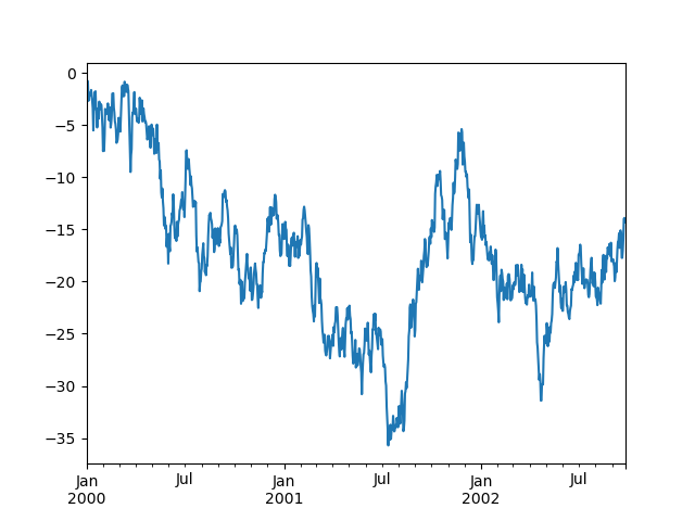
Plotting
Plotting docs.
In [130]: ts = pd.Series(np.random.randn(1000), index=pd.date_range('1/1/2000', periods=1000))

In [131]: ts = ts.cumsum()

In [132]: ts.plot()

Out[132]: <matplotlib.axes._subplots.AxesSubplot at 0x10efd5a90>
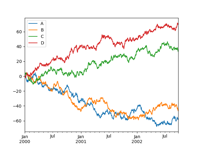
On DataFrame, plot() is a convenience to plot all of the columns with labels:
In [133]: df = pd.DataFrame(np.random.randn(1000, 4), index=ts.index,

   .....:                   columns=['A', 'B', 'C', 'D'])

   .....:

In [134]: df = df.cumsum()

In [135]: plt.figure(); df.plot(); plt.legend(loc='best')

Out[135]: <matplotlib.legend.Legend at 0x112854d90>
Getting Data In/Out
CSV
In [136]: df.to_csv('foo.csv')
In [137]: pd.read_csv('foo.csv')

Out[137]:

     Unnamed: 0          A          B         C          D

0    2000-01-01   0.266457  -0.399641 -0.219582   1.186860

1    2000-01-02  -1.170732  -0.345873  1.653061  -0.282953

2    2000-01-03  -1.734933   0.530468  2.060811  -0.515536

3    2000-01-04  -1.555121   1.452620  0.239859  -1.156896

4    2000-01-05   0.578117   0.511371  0.103552  -2.428202

5    2000-01-06   0.478344   0.449933 -0.741620  -1.962409

6    2000-01-07   1.235339  -0.091757 -1.543861  -1.084753

..          ...        ...        ...       ...        ...

993  2002-09-20 -10.628548  -9.153563 -7.883146  28.313940

994  2002-09-21 -10.390377  -8.727491 -6.399645  30.914107

995  2002-09-22  -8.985362  -8.485624 -4.669462  31.367740

996  2002-09-23  -9.558560  -8.781216 -4.499815  30.518439

997  2002-09-24  -9.902058  -9.340490 -4.386639  30.105593

998  2002-09-25 -10.216020  -9.480682 -3.933802  29.758560

999  2002-09-26 -11.856774 -10.671012 -3.216025  29.369368

[1000 rows x 5 columns]
HDF5
Reading and writing to HDFStores
Writing to a HDF5 Store
In [138]: df.to_hdf('foo.h5','df')
Reading from a HDF5 Store
In [139]: pd.read_hdf('foo.h5','df')

Out[139]:

                    A          B         C          D

2000-01-01   0.266457  -0.399641 -0.219582   1.186860

2000-01-02  -1.170732  -0.345873  1.653061  -0.282953

2000-01-03  -1.734933   0.530468  2.060811  -0.515536

2000-01-04  -1.555121   1.452620  0.239859  -1.156896

2000-01-05   0.578117   0.511371  0.103552  -2.428202

2000-01-06   0.478344   0.449933 -0.741620  -1.962409

2000-01-07   1.235339  -0.091757 -1.543861  -1.084753

...               ...        ...       ...        ...

2002-09-20 -10.628548  -9.153563 -7.883146  28.313940

2002-09-21 -10.390377  -8.727491 -6.399645  30.914107

2002-09-22  -8.985362  -8.485624 -4.669462  31.367740

2002-09-23  -9.558560  -8.781216 -4.499815  30.518439

2002-09-24  -9.902058  -9.340490 -4.386639  30.105593

2002-09-25 -10.216020  -9.480682 -3.933802  29.758560

2002-09-26 -11.856774 -10.671012 -3.216025  29.369368

[1000 rows x 4 columns]
Excel
Reading and writing to MS Excel
Writing to an excel file
In [140]: df.to_excel('foo.xlsx', sheet_name='Sheet1')
Reading from an excel file
In [141]: pd.read_excel('foo.xlsx', 'Sheet1', index_col=None, na_values=['NA'])

Out[141]:

                    A          B         C          D

2000-01-01   0.266457  -0.399641 -0.219582   1.186860

2000-01-02  -1.170732  -0.345873  1.653061  -0.282953

2000-01-03  -1.734933   0.530468  2.060811  -0.515536

2000-01-04  -1.555121   1.452620  0.239859  -1.156896

2000-01-05   0.578117   0.511371  0.103552  -2.428202

2000-01-06   0.478344   0.449933 -0.741620  -1.962409

2000-01-07   1.235339  -0.091757 -1.543861  -1.084753

...               ...        ...       ...        ...

2002-09-20 -10.628548  -9.153563 -7.883146  28.313940

2002-09-21 -10.390377  -8.727491 -6.399645  30.914107

2002-09-22  -8.985362  -8.485624 -4.669462  31.367740

2002-09-23  -9.558560  -8.781216 -4.499815  30.518439

2002-09-24  -9.902058  -9.340490 -4.386639  30.105593

2002-09-25 -10.216020  -9.480682 -3.933802  29.758560

2002-09-26 -11.856774 -10.671012 -3.216025  29.369368

[1000 rows x 4 columns]
Gotchas
If you are trying an operation and you see an exception like:
>>> if pd.Series([False, True, False]):

    print("I was true")

Traceback

    ...

ValueError: The truth value of an array is ambiguous. Use a.empty, a.any() or a.all().
See Comparisons for an explanation and what to do.
See Gotchas as well.
10分钟学习pandas的更多相关文章
- 10分钟了解 pandas - pandas官方文档译文 [原创]
10 Minutes to pandas 英文原文:https://pandas.pydata.org/pandas-docs/stable/10min.html 版本:pandas 0.23.4 采 ...
- 【译】10分钟学会Pandas
十分钟学会Pandas 这是关于Pandas的简短介绍主要面向新用户.你可以参考Cookbook了解更复杂的使用方法 习惯上,我们这样导入: In [1]: import pandas as pd I ...
- python 10分钟入门pandas
本文是对pandas官方网站上<10 Minutes to pandas>的一个简单的翻译,原文在这里.这篇文章是对pandas的一个简单的介绍,详细的介绍请参考:Cookbook .习惯 ...
- 十分钟(小时)学习pandas
十分钟学习pandas 一.导语 这篇文章从pandas官网翻译:链接,而且也有很多网友翻译过,而我为什么没去看他们的,而是去官网自己艰难翻译呢? 毕竟这是一个学习的过程,别人写的不如自己写的记忆深刻 ...
- 10分钟快速搞定pandas
本文是对pandas官方网站上<10 Minutes to pandas>的一个简单的翻译,原文在这里.这篇文章是对pandas的一个简单的介绍,详细的介绍请参考:Cookbook .习惯 ...
- Python数据分析Pandas库之熊猫(10分钟二)
pandas 10分钟教程(二) 重点发法 分组 groupby('列名') groupby(['列名1','列名2',.........]) 分组的步骤 (Splitting) 按照一些规则将数据分 ...
- Python数据分析Pandas库之熊猫(10分钟一)
pandas熊猫10分钟教程 排序 df.sort_index(axis=0/1,ascending=False/True) df.sort_values(by='列名') import numpy ...
- pandas入门10分钟——serries其实就是data frame的一列数据
10 Minutes to pandas This is a short introduction to pandas, geared mainly for new users. You can se ...
- Cookbook:pandas的学习之路——10 Minutes to pandas
按照pandas官网上10 Minutes to pandas的快速练习: 一 .对象创建: 导入练习所需要的工具包: 通过列表中的值创建序列Series,pandas在创建序列的同时会默认为列表中值 ...
随机推荐
- 简明 Git 命令速查表(中文版)
原文引用地址:https://github.com/flyhigher139/Git-Cheat-Sheet/blob/master/Git%20Cheat%20Sheet-Zh.md在Github上 ...
- Java中线程的生命周期
首先简单的介绍一下线程: 进程:正在运行中的程序.其实进程就是一个应用程序运行时的内存分配空间. 线程:其实就是进程中的一条执行路径.进程负责的是应用程序的空间的标示.线程负责的是应用程序的执行顺序. ...
- 谢欣伦 - OpenDev原创教程 - 本地IP查找类CxLocalHostIPAddrFind
这是一个精练的本地IP查找类,类名.函数名和变量名均采用匈牙利命名法.小写的x代表我的姓氏首字母(谢欣伦),个人习惯而已,如有雷同,纯属巧合. CxLocalHostIPAddrFind的使用如下: ...
- windows中查看开机时间
windows中查看开机时间 在windows下可以使用systeminfo命令来查看. 下面是网站摘录的关于windows启动了多长时间的内容 1. windows系统可以查看从开机到现在共 ...
- 如何使用Google Map API开发Android地图应用
两年前开发过的GoogleMap已经大变样,最近有项目要用到GoogleMap,重新来配置Android GoogleMap开发环境,还真是踩了不少坑. 一.下载Android SDK Manager ...
- Mac OS X:禁止崩溃报告-CrashReport
Mac OS X:禁止崩溃报告 崩溃报告就是CrashReport 至于官方的有关CrashReport的文档在Technical Note TN212 . 一般的默认情况下,当一个应用程序因为各种原 ...
- Spring整理
Bean配置 1. <context:component-scan base-package="com.test" />这个包下的Spring注解才有效 属性文件自动解 ...
- maven---install报错
若maven项目在install或者run的时候出现莫名奇妙的问题,应该考虑是否在pom.xml中引入的包是否为最新的包: 因为在本地maven仓库中已经存在的包就不会再下载,所以可以从这方面排查问题 ...
- 使用postman发送数据并构建collections执行测试
1.安装 下载地址:https://www.getpostman.com/.直接安装,成功后在chorme的应用程序中会多出一个Postman.如果无法在google store上直接安装,可以下载. ...
- Selenium2学习-042-Selenium3启动Firefox Version 48.x浏览器(ff 原生 geckodriver 诞生)
今天又被坑了一把,不知谁把 Slave 机的火狐浏览器版本升级为了 48 的版本,导致网页自动化测试脚本无法启动火狐的浏览器,相关的网页自动化脚本全线飘红(可惜不是股票,哈哈哈...),报版本不兼容的 ...