MATLAB实例：PCA（主成成分分析）详解

MATLAB实例：PCA（主成成分分析）详解

作者：凯鲁嘎吉 - 博客园 http://www.cnblogs.com/kailugaji/

1. 主成成分分析

2. MATLAB解释

详细信息请看：Principal component analysis of raw data - mathworks

[coeff,score,latent,tsquared,explained,mu] = pca(X)

coeff = pca(X) returns the principal component coefficients, also known as loadings, for the n-by-p data matrix X. Rows of X correspond to observations and columns correspond to variables.

The coefficient matrix is p-by-p.

Each column of coeff contains coefficients for one principal component, and the columns are in descending order of component variance.

By default, pca centers the data and uses the singular value decomposition (SVD) algorithm.

coeff = pca(X,Name,Value) returns any of the output arguments in the previous syntaxes using additional options for computation and handling of special data types, specified by one or more Name,Value pair arguments.

For example, you can specify the number of principal components pca returns or an algorithm other than SVD to use.

[coeff,score,latent] = pca(___) also returns the principal component scores in score and the principal component variances in latent.

You can use any of the input arguments in the previous syntaxes.

Principal component scores are the representations of X in the principal component space. Rows of score correspond to observations, and columns correspond to components.

The principal component variances are the eigenvalues of the covariance matrix of X.

[coeff,score,latent,tsquared] = pca(___) also returns the Hotelling's T-squared statistic for each observation in X.

[coeff,score,latent,tsquared,explained,mu] = pca(___) also returns explained, the percentage of the total variance explained by each principal component and mu, the estimated mean of each variable in X.

coeff: X矩阵所对应的协方差矩阵的所有特征向量组成的矩阵，即变换矩阵或投影矩阵，coeff每列代表一个特征值所对应的特征向量，列的排列方式对应着特征值从大到小排序。

source: 表示原数据在各主成分向量上的投影。但注意：是原数据经过中心化后在主成分向量上的投影。

latent: 是一个列向量，主成分方差，也就是各特征向量对应的特征值，按照从大到小进行排列。

tsquared: X中每个观察值的Hotelling的T平方统计量。Hotelling的T平方统计量（T-Squared Statistic）是每个观察值的标准化分数的平方和，以列向量的形式返回。

explained: 由每个主成分解释的总方差的百分比，每一个主成分所贡献的比例。explained = 100*latent/sum(latent)。

mu: 每个变量X的估计平均值。

3. MATLAB程序

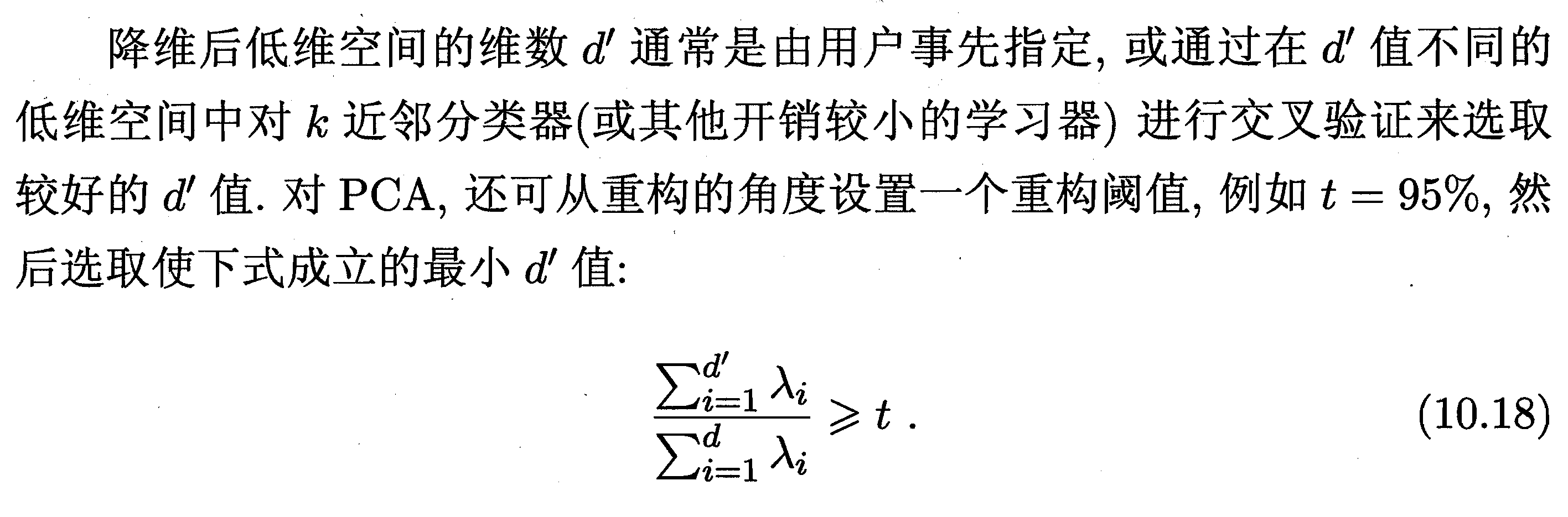
3.1 方法一：指定降维后低维空间的维度k

function [data_PCA, COEFF, sum_explained]=pca_demo_1(data,k)
% k:前k个主成分
data=zscore(data);  %归一化数据
[COEFF,SCORE,latent,tsquared,explained,mu]=pca(data);
latent1=100*latent/sum(latent);%将latent特征值总和统一为100，便于观察贡献率
data= bsxfun(@minus,data,mean(data,1));
data_PCA=data*COEFF(:,1:k);
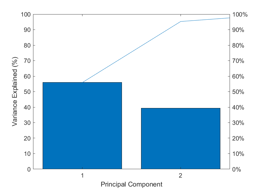
pareto(latent1);%调用matla画图 pareto仅绘制累积分布的前95%，因此y中的部分元素并未显示
xlabel('Principal Component');
ylabel('Variance Explained (%)');
% 图中的线表示的累积变量解释程度
print(gcf,'-dpng','PCA.png');
sum_explained=sum(explained(1:k));

3.2 方法二：指定贡献率percent_threshold

function [data_PCA, COEFF, sum_explained, n]=pca_demo_2(data)
%用percent_threshold决定保留xx%的贡献率
percent_threshold=95;   %百分比阈值，用于决定保留的主成分个数；
data=zscore(data);  %归一化数据
[COEFF,SCORE,latent,tsquared,explained,mu]=pca(data);
latent1=100*latent/sum(latent);%将latent特征值总和统一为100，便于观察贡献率
A=length(latent1);
percents=0;                          %累积百分比
for n=1:A
    percents=percents+latent1(n);
    if percents>percent_threshold
        break;
    end
end
data= bsxfun(@minus,data,mean(data,1));
data_PCA=data*COEFF(:,1:n);
pareto(latent1);%调用matla画图 pareto仅绘制累积分布的前95%，因此y中的部分元素并未显示
xlabel('Principal Component');
ylabel('Variance Explained (%)');
% 图中的线表示的累积变量解释程度
print(gcf,'-dpng','PCA.png');
sum_explained=sum(explained(1:n));

4. 结果

数据来源于MATLAB自带的数据集hald

>> load hald
>> [data_PCA, COEFF, sum_explained]=pca_demo_1(ingredients,2)

data_PCA =

  -1.467237802258083  -1.903035708425560
  -2.135828746398875  -0.238353702721984
   1.129870473833422  -0.183877154192583
  -0.659895489750766  -1.576774209965747
   0.358764556470351  -0.483537878558994
   0.966639639692207  -0.169944028103651
   0.930705117077330   2.134816511997477
  -2.232137996884836   0.691670682875924
  -0.351515595975561   1.432245069443404
   1.662543014130206  -1.828096643220118
  -1.640179952926685   1.295112751426928
   1.692594091826333   0.392248821530480
   1.745678691164958   0.437525487914425

COEFF =

   0.475955172748970  -0.508979384806410   0.675500187964285   0.241052184051094
   0.563870242191994   0.413931487136985  -0.314420442819292   0.641756074427213
  -0.394066533909303   0.604969078471439   0.637691091806566   0.268466110294533
  -0.547931191260863  -0.451235109330016  -0.195420962611708   0.676734019481284

sum_explained =

  95.294252628439153

>> [data_PCA, COEFF, sum_explained, n]=pca_demo_2(ingredients)

data_PCA =

  -1.467237802258083  -1.903035708425560
  -2.135828746398875  -0.238353702721984
   1.129870473833422  -0.183877154192583
  -0.659895489750766  -1.576774209965747
   0.358764556470351  -0.483537878558994
   0.966639639692207  -0.169944028103651
   0.930705117077330   2.134816511997477
  -2.232137996884836   0.691670682875924
  -0.351515595975561   1.432245069443404
   1.662543014130206  -1.828096643220118
  -1.640179952926685   1.295112751426928
   1.692594091826333   0.392248821530480
   1.745678691164958   0.437525487914425

COEFF =

   0.475955172748970  -0.508979384806410   0.675500187964285   0.241052184051094
   0.563870242191994   0.413931487136985  -0.314420442819292   0.641756074427213
  -0.394066533909303   0.604969078471439   0.637691091806566   0.268466110294533
  -0.547931191260863  -0.451235109330016  -0.195420962611708   0.676734019481284

sum_explained =

  95.294252628439153

n =

     2

5. 参考

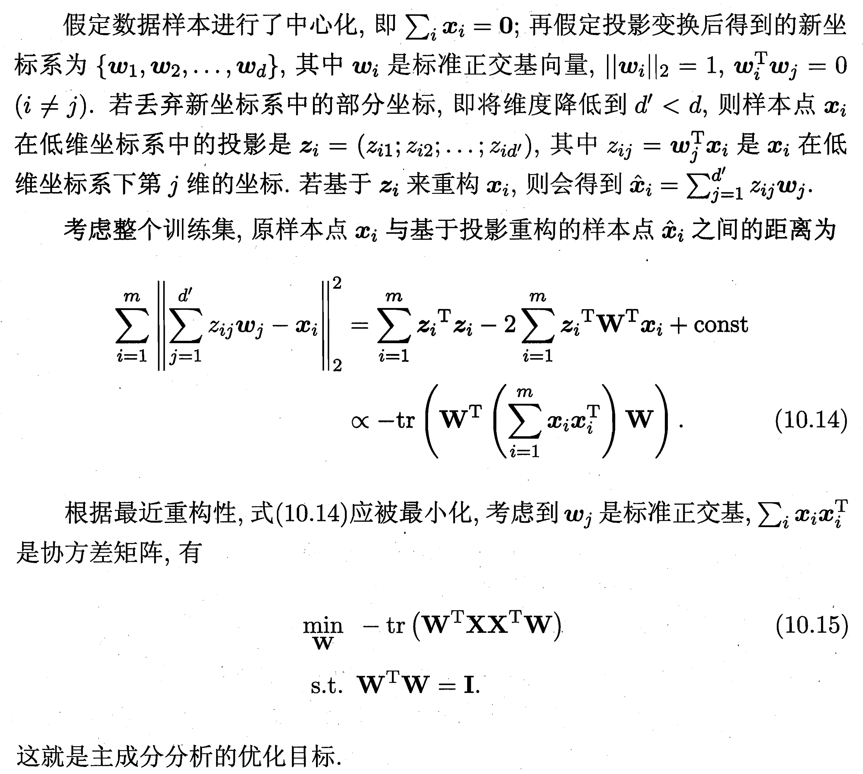
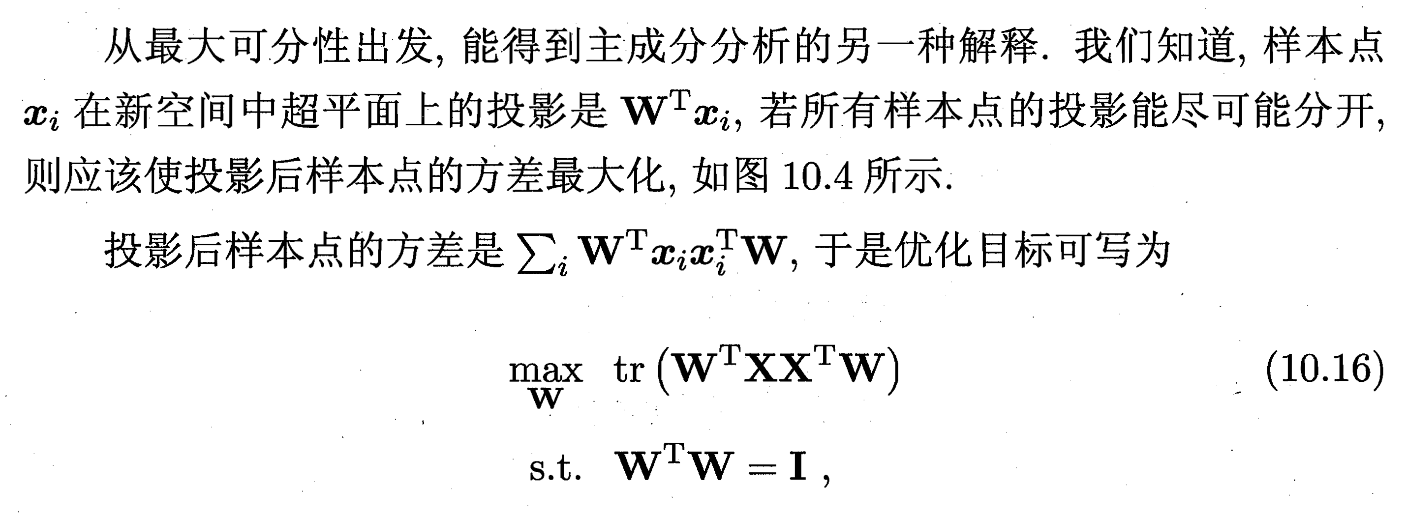
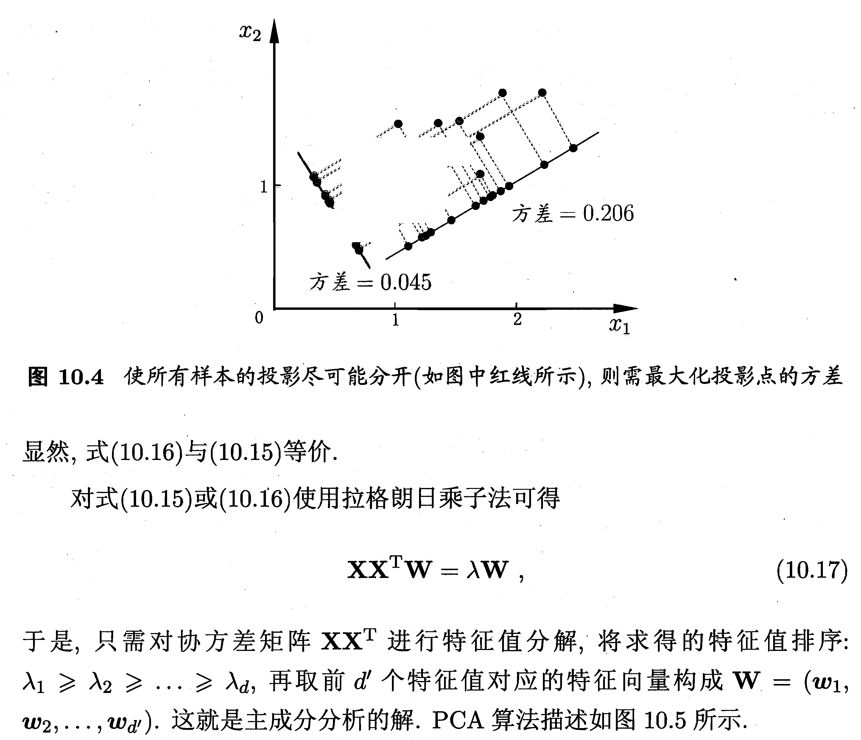
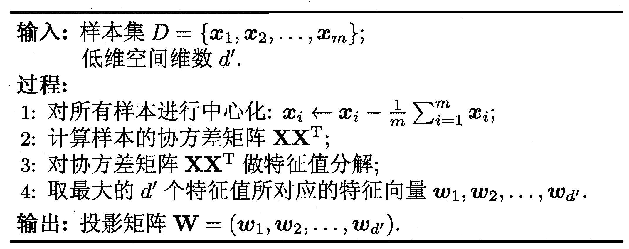
[1] 周志华,《机器学习》.

[2] MATLAB实例：PCA降维