linux上搭建单机版hadoop和spark
楔子
这一次我们来用pandas实现一下SQL中的窗口函数,所以也会介绍关于SQL窗口函数的一些知识,以下SQL语句运行在PostgreSQL上。
数据集
select * from sales_data

-- 字段名分别是:saledate(销售日期)、product(商品)、channel(销售渠道)、amount(销售金额)

/*

2019-01-01	桔子	淘宝	1864

2019-01-01	桔子	京东	1329

2019-01-01	桔子	店面	1736

2019-01-01	香蕉	淘宝	1573

2019-01-01	香蕉	京东	1364

2019-01-01	香蕉	店面	1178

2019-01-01	苹果	淘宝	511

2019-01-01	苹果	京东	568

2019-01-01	苹果	店面	847

2019-01-02	桔子	淘宝	1923

2019-01-02	桔子	京东	775

2019-01-02	桔子	店面	599

2019-01-02	香蕉	淘宝	1612

2019-01-02	香蕉	京东	1057

2019-01-02	香蕉	店面	1580

2019-01-02	苹果	淘宝	1345

2019-01-02	苹果	京东	564

2019-01-02	苹果	店面	1953

2019-01-03	桔子	淘宝	729

2019-01-03	桔子	京东	1758

2019-01-03	桔子	店面	918

2019-01-03	香蕉	淘宝	1879

2019-01-03	香蕉	京东	1142

2019-01-03	香蕉	店面	731

2019-01-03	苹果	淘宝	1329

2019-01-03	苹果	京东	1315

2019-01-03	苹果	店面	1956

*/
移动分析和累计求和
这里我们需要说一下什么是窗口函数,窗口函数和聚合函数类似,都是针对一组数据进行分析计算;但不同的是,聚合函数是将一组数据汇总成单个结果,窗口函数是为每一行数据都返回一个汇总后的结果
我们用一张图来说明一下:

可以看到:聚合函数会将同一个组内的多条数据汇总成一条数据,但是窗口函数保留了所有的原始数据。
窗口函数也被称为联机分析处理(OLAP)函数,或者分析函数(Analytic Function)。
我们以 SUM 函数为例,比较这两种函数的差异。
select sum(amount) as sum_amount

from sales_data where saledate = '2019-01-01';

/*

10970

*/

-- 我们说一旦出现了聚合函数,那么select后面的字段要么出现在聚合函数中,要么出现在group by字句中

-- 但对于窗口函数则不需要

select saledate, product, sum(amount) over() as sum_amount

from sales_data

where saledate = '2019-01-01'

/*

2019-01-01	桔子	10970

2019-01-01	桔子	10970

2019-01-01	桔子	10970

2019-01-01	香蕉	10970

2019-01-01	香蕉	10970

2019-01-01	香蕉	10970

2019-01-01	苹果	10970

2019-01-01	苹果	10970

2019-01-01	苹果	10970

*/
OVER 关键字表明 SUM 是一个窗口函数;括号内为空表示将所有数据作为整体进行分析。
查询结果返回了所有的记录,并且 SUM 聚合函数为每条记录都返回了相同的汇总结果。
从上面的示例可以看出,窗口函数与其他函数的不同之处在于它包含了一个 OVER 子句;OVER 子句用于定义一个分析数据的窗口。完整的窗口函数定义如下:
window_function ( expression ) OVER (

    PARTITION BY ...

    ORDER BY ...

    frame_clause

)
其中,window_function 是窗口函数的名称;expression 是窗口函数操作的对象,可以是字段或者表达式;OVER 子句包含三个部分:分区(PARTITION BY)、排序(ORDER BY)以及窗口大小(frame_clause)
在介绍这些组成之前,我们先来看看上面那个例子使用pandas如何实现:
import pandas as pd

from sqlalchemy import create_engine

engine = create_engine("postgres://postgres:zgghyys123@localhost:5432/postgres")

df = pd.read_sql("select saledate, product, amount from sales_data where saledate = '2019-01-01'",engine)

# 这个实现起来显然很容易

df["amount"] = df["amount"].sum()

print(df)

"""

     saledate    product  amount

0  2019-01-01      桔子   10970

1  2019-01-01      桔子   10970

2  2019-01-01      桔子   10970

3  2019-01-01      香蕉   10970

4  2019-01-01      香蕉   10970

5  2019-01-01      香蕉   10970

6  2019-01-01      苹果   10970

7  2019-01-01      苹果   10970

8  2019-01-01      苹果   10970

"""
下面来看看这些选项的作用
分区(PARTITION BY)
OVER 子句中的 PARTITION BY 选项用于定义分区,作用类似于 GROUP BY 分组;如果指定了分区选项,窗口函数将会分别针对每个分区单独进行分析。
select saledate, product, sum(amount) over(partition by product) as sum_amount

from sales_data

where saledate = '2019-01-01'
我们看到窗口函数会针对partition by后面字段进行分区,相同的分为一个区,然后对每个分区里面的值进行计算。我们按照product进行分区,那么所有值为"桔子"的分为一区,那么它的sum_amount就是所有product为"桔子"的amount之和,同理苹果、香蕉也是如此。
我们看到窗口函数,虽然也用到了聚合,但是它并不需要group by,因为字段的数量和原来保持一致。只是针对partition by后面的字段进行分区,然后对每一个区使用聚合得到一个值,然后给该分区的所有记录都添上这么一个值。
现在再回来看开始的例子,saledate='2019-01-01'的记录有10条,那么select sum(amount) from sale_data saledate='2019-01-01'得到的数据只有一条,也就是所有的amount之和。而select sum(amount) over() from sale_data saledate='2019-01-01',我们说由于over()里面是空的,所以相当于整体只有一个分区,这个分区就是整个筛选出来的数据集,那么还是计算所有的amount之和,但是返回的是10条,和原来的数据行数保持一致。
并且窗口函数不需要group by,前面可以直接加上指定的字段,还是那句话,它不改变数据集的大小,而是在聚合之后给原来的每一条记录都添上这么一个值。但是普通的聚合就不行了,如果select指定了其它字段,那么这些字段必须出现在聚合函数、或者group by字句中,并且计算完之后数据行数会减少(除非group by后面的字段都不重复,但如果不重复的话,我们一般也不会用它来group by)
然后我们看一下如何使用pandas来实现
df = pd.read_sql("select saledate, product, amount from sales_data where saledate = '2019-01-01'",engine)
# pandas实现SQL的聚合函数和窗口函数都使用groupby函数
groupby = df.groupby(by=["product"])
# 如果后面调用了agg,那么等价于SQL的聚合函数。如果是transform,那么就等价于SQL的窗口函数
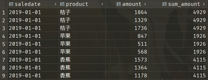
df["sum_amount"] = groupby["amount"].transform("sum")
print(df)
"""
saledate product amount sum_amount
0 2019-01-01 桔子 1864 4929
1 2019-01-01 桔子 1329 4929
2 2019-01-01 桔子 1736 4929
3 2019-01-01 香蕉 1573 4115
4 2019-01-01 香蕉 1364 4115
5 2019-01-01 香蕉 1178 4115
6 2019-01-01 苹果 511 1926
7 2019-01-01 苹果 568 1926
8 2019-01-01 苹果 847 1926
"""
# 虽然顺序不同,但是结果是一致的。
partition by后面可以指定多个字段,比如:
select saledate, product, amount, sum(amount) over(partition by saledate, product) as sum_amount

from sales_data

/*

2019-01-01	桔子	1329	4929

2019-01-01	桔子	1736	4929

2019-01-01	桔子	1864	4929

2019-01-01	苹果	568	1926

2019-01-01	苹果	511	1926

2019-01-01	苹果	847	1926

2019-01-01	香蕉	1178	4115

2019-01-01	香蕉	1573	4115

2019-01-01	香蕉	1364	4115

2019-01-02	桔子	775	3297

2019-01-02	桔子	1923	3297

2019-01-02	桔子	599	3297

2019-01-02	苹果	1953	3862

2019-01-02	苹果	564	3862

2019-01-02	苹果	1345	3862

2019-01-02	香蕉	1057	4249

2019-01-02	香蕉	1612	4249

2019-01-02	香蕉	1580	4249

2019-01-03	桔子	729	3405

2019-01-03	桔子	1758	3405

2019-01-03	桔子	918	3405

2019-01-03	苹果	1956	4600

2019-01-03	苹果	1329	4600

2019-01-03	苹果	1315	4600

2019-01-03	香蕉	1879	3752

2019-01-03	香蕉	1142	3752

2019-01-03	香蕉	731	3752

*/
我们看到,partition by后面指定了saledate、product,那么相当于按照sale、product进行分区,相同的分为一区。然后对每一个分区里面的amount进行求和,然后给该分区里面的所有的行都添上求和之后的值。所以2019-01-01 桔子对应的sum_amount是4929,因为所有2019-01-01 桔子 对应的amount加起来是5929,然后给这个分区对应的每条记录都添上4929这个值。同理对于其它的记录也是同样的道理。
对于pandas而言,只需要再groupby中多指定一个字段即可
df = pd.read_sql("select saledate, product, amount from sales_data",engine)

groupby = df.groupby(by=["saledate", "product"])

df["sum_amount"] = groupby["amount"].transform("sum")

print(df)

"""

     saledate   product  amount  sum_amount

0   2019-01-01      桔子    1864        4929

1   2019-01-01      桔子    1329        4929

2   2019-01-01      桔子    1736        4929

3   2019-01-01      香蕉    1573        4115

4   2019-01-01      香蕉    1364        4115

5   2019-01-01      香蕉    1178        4115

6   2019-01-01      苹果     511        1926

7   2019-01-01      苹果     568        1926

8   2019-01-01      苹果     847        1926

9   2019-01-02      桔子    1923        3297

10  2019-01-02      桔子     775        3297

11  2019-01-02      桔子     599        3297

12  2019-01-02      香蕉    1612        4249

13  2019-01-02      香蕉    1057        4249

14  2019-01-02      香蕉    1580        4249

15  2019-01-02      苹果    1345        3862

16  2019-01-02      苹果     564        3862

17  2019-01-02      苹果    1953        3862

18  2019-01-03      桔子     729        3405

19  2019-01-03      桔子    1758        3405

20  2019-01-03      桔子     918        3405

21  2019-01-03      香蕉    1879        3752

22  2019-01-03      香蕉    1142        3752

23  2019-01-03      香蕉     731        3752

24  2019-01-03      苹果    1329        4600

25  2019-01-03      苹果    1315        4600

26  2019-01-03      苹果    1956        4600

"""
在窗口函数中指定 PARTITION BY 选项之后,不需要 GROUP BY 子句也能获得分组统计信息。如果不指定 PARTITION BY 选项,所有的数据作为一个整体进行分析。
排序(ORDER BY)
OVER 子句中的 ORDER BY 选项用于指定分区内的排序方式,与 ORDER BY 子句的作用类似;排序选项通常用于数据的排名分析。
partition by ... order by ... [asc|desc]
排序也是可以指定多个字段进行排序的,多个字段逗号分隔,order by要在partition by的后面。并且排序也是针对自身所在的分区来的,每个分区的内部进行排序。
我们现在知道了,partition by是根据指定字段分区,然后对每个分区使用前面的函数,忘记说了,over()前面必须是函数,比如:sum(amount) over(),不可以是amount over()。然后order by是根据指定字段,对分区里面的记录进行排序。可以只指定partition by不指定order by,我们前面已经见过了。当然也可以只指定order by,不指定partition by。我们先来看看只指定order by,不指定partition by的话,会是什么结果。
select amount, sum(amount) over(order by amount) as sum_amount

from sales_data where saledate = '2019-01-01';

/*

511	511

568	1079

847	1926

1178	3104

1329	4433

1364	5797

1573	7370

1736	9106

1864	10970

*/

select amount, sum(amount) over(order by amount desc) as sum_amount

from sales_data where saledate = '2019-01-01';

/*

1864	1864

1736	3600

1573	5173

1364	6537

1329	7866

1178	9044

847	9891

568	10459

511	10970

*/
我们看到实现了累加的效果,我们知道指定partition by,那么根据哪些字段分区是由partition by后面的字段决定的。但如果在不指定partition by、只指定order by的情况下,那么就只有一个分区,这个分区就是全部记录,然后会根据order by后面的字段对全部记录进行排序,然后再进行累和(假设是对于sum而言,其它的函数也是类似的),所以第2行的值等于原来第1行的值加上原来第2行的值。
我们目前是按照amount进行order by,而amount没有重复的,所以是逐行累加。如果我们是根据product进行order by的话会咋样呢?product是有重复的
select product, amount, sum(amount) over(order by product) as sum_amount

from sales_data where saledate = '2019-01-01';

/*

桔子	1864	4929

桔子	1329	4929

桔子	1736	4929

苹果	847	6855

苹果	511	6855

苹果	568	6855

香蕉	1573	10970

香蕉	1364	10970

香蕉	1178	10970

*/
我们说order by是先排序,这是按照product排序,显然是按照其拼音首字符的ascii码进行排序。当然排序不重要,重点是后面的累加。我们看到并没有逐行累加,而是把product相同的先分别加在一起,得到的结果是:桔子:5929 苹果: 1926 香蕉:4115,然后再对整体进行累加,所以苹果的值应该是:5929+1926=7855,同理香蕉的值:5929+1926+4115=11970。
所以这个累加并不是针对每一行来的,而是先把product相同的amount都加在一起,然后对加在一起的值进行累加。并且累加之后,再将累加的的结果添加到对应product的每一条记录上。而我们上面第一个例子之所以是逐行累加,是因为我们order by指定的是amount,而amount都不重复。
然后我们再来看看pandas如何实现这个逻辑
df = pd.read_sql("select product, amount from sales_data where saledate = '2019-01-01'", engine)

# 如果是实现over(order by)的话,不需要使用groupby

df = df.sort_values(by=["amount"])

df["sum_amount"] = df["amount"].agg("cumsum")

print(df)

"""

    product  amount  sum_amount

6      苹果     511         511

7      苹果     568        1079

8      苹果     847        1926

5      香蕉    1178        3104

1      桔子    1329        4433

4      香蕉    1364        5797

3      香蕉    1573        7370

2      桔子    1736        9106

0      桔子    1864       10970

"""
倒序排序也是可以的
df = pd.read_sql("select product, amount from sales_data where saledate = '2019-01-01'", engine)

df = df.sort_values(by=["amount"], ascending=False)

df["sum_amount"] = df["amount"].agg("cumsum")

print(df)

"""

    product  amount  sum_amount

0      桔子    1864        1864

2      桔子    1736        3600

3      香蕉    1573        5173

4      香蕉    1364        6537

1      桔子    1329        7866

5      香蕉    1178        9044

8      苹果     847        9891

7      苹果     568       10459

6      苹果     511       10970

"""
我们这里amount没有重复的,所以得到的结果和SQL是一样的,但如果是product呢?
df = df.sort_values(by=["product"])

df["sum_amount"] = df["amount"].agg("cumsum")

print(df)

"""

    product  amount  sum_amount

0      桔子    1864        1864

1      桔子    1329        3193

2      桔子    1736        4929

6      苹果     511        5440

7      苹果     568        6008

8      苹果     847        6855

3      香蕉    1573        8428

4      香蕉    1364        9792

5      香蕉    1178       10970

"""
我们看到结果和SQL有些不一样,SQL是先将amount按照product相同的加在一起,然后再进行累加,而pandas依旧是逐行累加。那么如何实现SQL的逻辑呢?
df = pd.read_sql("select product, amount from sales_data where saledate = '2019-01-01'", engine)

df = df.sort_values(by=["product"])

df["sum_amount"] = df.groupby(by=["product"])["amount"].transform("sum")

print(df)

"""

    product  amount  sum_amount

0      桔子    1864        4929

1      桔子    1329        4929

2      桔子    1736        4929

6      苹果     511        1926

7      苹果     568        1926

8      苹果     847        1926

3      香蕉    1573        4115

4      香蕉    1364        4115

5      香蕉    1178        4115

"""

# 实现了按照product相同的先加在一起,但是还没有实现累和

# 苹果的sum_amount应该是4929 + 1926,香蕉的sum_amount应该是4929 + 1926 + 4115

tmp = df.drop_duplicates(["product"])[["product", "sum_amount"]]

tmp["sum_amount"] = tmp["sum_amount"].cumsum()

print(tmp)

"""

    product  sum_amount

0      桔子        4929

6      苹果        6855

3      香蕉       10970

"""

print(

    pd.merge(df.drop(columns=["sum_amount"]), tmp, on="product", how="left")

)

"""

    product  amount  sum_amount

0      桔子    1864        4929

1      桔子    1329        4929

2      桔子    1736        4929

6      苹果     511        6855

7      苹果     568        6855

8      苹果     847        6855

3      香蕉    1573       10970

4      香蕉    1364       10970

5      香蕉    1178       10970

"""
所以我们看到over里面的order by实现的就是先排序再累加的效果,只不过这个累加会先根据order by后面的字段中值相同的进行求和,然后再累加。
单独指定partition by和单独指定order by我们已经知道了,但如果partition by和order by同时指定的话会怎么样呢?
select product, amount, sum(amount) over (partition by product order by amount desc) as sum_amount

from sales_data

where saledate = '2019-01-01';

/*

桔子	1864	1864

桔子	1736	3600

桔子	1329	4929

苹果	847	847

苹果	568	1415

苹果	511	1926

香蕉	1573	1573

香蕉	1364	2937

香蕉	1178	4115

*/
我们看到是按照product分区,按照amount排序,但此时依旧出现了累和(我们以前面的聚合是sum为例),但显然它是在分区内部进行累和。我们知道如果不指定partition by的话,那么order by amount会对整个数据集进行排序,然后进行累和。但是现在指定partition by了,那么会先根据partition by进行分区,然后order by的逻辑还是跟之前一样,可以认为是在各自的分区内部分别执行了order by。
然后看看pandas如何实现
df = pd.read_sql("select product, amount from sales_data where saledate = '2019-01-01'", engine)

groupby = df.groupby(by=["product"])

df["sum_amount"] = groupby["amount"].transform("cumsum")

print(df)

"""

    product  amount  sum_amount

0      桔子    1864        1864

1      桔子    1329        3193

2      桔子    1736        4929

3      香蕉    1573        1573

4      香蕉    1364        2937

5      香蕉    1178        4115

6      苹果     511         511

7      苹果     568        1079

8      苹果     847        1926

"""
由于排序不一样,导致每个分区内amount的顺序不一样,但结果是正确的。我们再来看个栗子:
select product, saledate, amount, sum(amount) over (partition by product order by saledate) as sum_amount

from sales_data;

/*

桔子	2019-01-01	1864	4929

桔子	2019-01-01	1329	4929

桔子	2019-01-01	1736	4929

桔子	2019-01-02	599	8226

桔子	2019-01-02	775	8226

桔子	2019-01-02	1923	8226

桔子	2019-01-03	729	11631

桔子	2019-01-03	918	11631

桔子	2019-01-03	1758	11631

苹果	2019-01-01	847	1926

苹果	2019-01-01	568	1926

苹果	2019-01-01	511	1926

苹果	2019-01-02	564	5788

苹果	2019-01-02	1953	5788

苹果	2019-01-02	1345	5788

苹果	2019-01-03	1956	10388

苹果	2019-01-03	1329	10388

苹果	2019-01-03	1315	10388

香蕉	2019-01-01	1573	4115

香蕉	2019-01-01	1178	4115

香蕉	2019-01-01	1364	4115

香蕉	2019-01-02	1612	8364

香蕉	2019-01-02	1580	8364

香蕉	2019-01-02	1057	8364

香蕉	2019-01-03	1879	12116

香蕉	2019-01-03	1142	12116

香蕉	2019-01-03	731	12116

*/
以桔子为例,这个结果像不像我们单独使用order by的时候所得到的结果呢?我们是按照product分区的,相同的product归为一个区。然后在各自的分区里面,先通过order by saledate进行排序,再把saledate相同的amount先进行求和,以桔子为例:2019-01-01的amount总和是5929,2019-01-02的amount总和是3297,然后累加,2019-01-02的amount总和就是5929+3297=9226,同理3号的逻辑也是如此。所以我们看到order by的逻辑不变,如果没有partition by,那么它的作用范围就是整个数据集、因为此时整体是一个分区;如果有partition by,那么在分区之后,order by的作用范围就是一个个的分区,就把每一个分区想象成独立的数据集就行,在各自的分区内部执行order by的逻辑。同理下面的苹果和香蕉也是一样的逻辑。
然后使用pandas实现,会稍微麻烦一些:
df = pd.read_sql("select product, saledate, amount from sales_data", engine)

# 执行groupby

groupby = df.groupby(by=["product", "saledate"])

df["sum_amount"] = groupby["amount"].transform("sum")

print(df)

"""

     product    saledate  amount  sum_amount

0       桔子  2019-01-01    1864        4929

1       桔子  2019-01-01    1329        4929

2       桔子  2019-01-01    1736        4929

3       香蕉  2019-01-01    1573        4115

4       香蕉  2019-01-01    1364        4115

5       香蕉  2019-01-01    1178        4115

6       苹果  2019-01-01     511        1926

7       苹果  2019-01-01     568        1926

8       苹果  2019-01-01     847        1926

9       桔子  2019-01-02    1923        3297

10      桔子  2019-01-02     775        3297

11      桔子  2019-01-02     599        3297

12      香蕉  2019-01-02    1612        4249

13      香蕉  2019-01-02    1057        4249

14      香蕉  2019-01-02    1580        4249

15      苹果  2019-01-02    1345        3862

16      苹果  2019-01-02     564        3862

17      苹果  2019-01-02    1953        3862

18      桔子  2019-01-03     729        3405

19      桔子  2019-01-03    1758        3405

20      桔子  2019-01-03     918        3405

21      香蕉  2019-01-03    1879        3752

22      香蕉  2019-01-03    1142        3752

23      香蕉  2019-01-03     731        3752

24      苹果  2019-01-03    1329        4600

25      苹果  2019-01-03    1315        4600

26      苹果  2019-01-03    1956        4600

"""

tmp = df.drop_duplicates(["product", "saledate", "sum_amount"])

tmp["sum_amount"] = tmp.groupby(by=["product"])["sum_amount"].transform("cumsum")

print(tmp)

"""

    product    saledate  amount  sum_amount

0       桔子  2019-01-01    1864        4929

3       香蕉  2019-01-01    1573        4115

6       苹果  2019-01-01     511        1926

9       桔子  2019-01-02    1923        8226

12      香蕉  2019-01-02    1612        8364

15      苹果  2019-01-02    1345        5788

18      桔子  2019-01-03     729       11631

21      香蕉  2019-01-03    1879       12116

24      苹果  2019-01-03    1329       10388

"""

print(

    pd.merge(

        df.drop(columns=["sum_amount", "amount"]), tmp, on=["product", "saledate"], how="left"

    ).sort_values(by=["product", "saledate"])

)

"""

   product    saledate  amount  sum_amount

0       桔子  2019-01-01    1864        4929

1       桔子  2019-01-01    1864        4929

2       桔子  2019-01-01    1864        4929

9       桔子  2019-01-02    1923        8226

10      桔子  2019-01-02    1923        8226

11      桔子  2019-01-02    1923        8226

18      桔子  2019-01-03     729       11631

19      桔子  2019-01-03     729       11631

20      桔子  2019-01-03     729       11631

6       苹果  2019-01-01     511        1926

7       苹果  2019-01-01     511        1926

8       苹果  2019-01-01     511        1926

15      苹果  2019-01-02    1345        5788

16      苹果  2019-01-02    1345        5788

17      苹果  2019-01-02    1345        5788

24      苹果  2019-01-03    1329       10388

25      苹果  2019-01-03    1329       10388

26      苹果  2019-01-03    1329       10388

3       香蕉  2019-01-01    1573        4115

4       香蕉  2019-01-01    1573        4115

5       香蕉  2019-01-01    1573        4115

12      香蕉  2019-01-02    1612        8364

13      香蕉  2019-01-02    1612        8364

14      香蕉  2019-01-02    1612        8364

21      香蕉  2019-01-03    1879       12116

22      香蕉  2019-01-03    1879       12116

23      香蕉  2019-01-03    1879       12116

"""
指定窗口大小
指定窗口大小稍微有点复杂,可能需要花点时间来理解,与其说复杂,倒不如说东西有点多。可能开始不理解,但是坚持看完,你肯定会明白的,不要看到一半就放弃了,一定要看完,因为通过后面的例子、以及解释会对开始的内容进行补充和呼应。
OVER 子句中的 frame_clause 选项用于指定一个移动的窗口。窗口总是位于分区范围之内,是分区的一个子集。指定了窗口之后,函数不再基于分区进行计算,而是基于窗口内的数据进行计算。窗口选项可以实现许多复杂的计算。例如,累计到当前日期为止的销量总计,每个月份及其前后各一月(3 个月)的平均销量等。窗口大小的具体选项如下:
ROWS frame_start

-- 或者

ROWS BETWEEN frame_start AND frame_end
其中,ROWS 表示以行为单位计算窗口的偏移量。frame_start 用于定义窗口的起始位置,可以指定以下内容之一:
- UNBOUNDED PRECEDING,窗口从分区的第一行开始,默认值;
- N PRECEDING,窗口从当前行之前的第 N 行开始;
- CURRENT ROW,窗口从当前行开始。
frame_end 用于定义窗口的结束位置,可以指定以下内容之一:
- CURRENT ROW,窗口到当前行结束,默认值;
- N FOLLOWING,窗口到当前行之后的第 N 行结束。
- UNBOUNDED FOLLOWING,窗口到分区的最后一行结束;
下图演示了这些窗口选项的作用:

窗口函数依次处理每一行数据,CURRENT ROW 表示当前正在处理的数据;其他的行可以使用相对当前行的位置表示。需要注意的是,窗口的大小不会超出分区的范围。
窗口函数的选项比较复杂,我们通过一些常见的窗口函数示例来理解它们的作用。常见的窗口函数可以分为以下几类:聚合窗口函数、排名窗口函数以及取值窗口函数。
许多聚合函数也可以作为窗口函数使用,包括 AVG、SUM、COUNT、MAX 以及 MIN 等。
-- 本来order by amount是按对每个分区内部的记录进行累加的,当然这里的累加并不是逐行累加,是我们上面说的那样

-- 只是为了方便,我们就直接说累加了,或者累和也是一样,因为我们这里是以sum函数为例子

-- 但是我们指定了窗口大小,那么怎么加就由我们指定的窗口大小来决定了,而不是整个分区

select product, amount,

       sum(amount) over(partition by product order by amount rows unbounded preceding) as sum_amount

from sales_data where saledate = '2019-01-01';

/*

桔子	1329	1329

桔子	1736	3065

桔子	1864	4929

苹果	511	511

苹果	568	1079

苹果	847	1926

香蕉	1178	1178

香蕉	1364	2542

香蕉	1573	4115

*/
OVER 子句中的 PARTITION BY 选项表示按照product进行分区,ORDER BY 选项表示按照amount进行排序。窗口子句 ROWS UNBOUNDED PRECEDING 指定窗口从分区的第一行开始,默认到当前行结束;也就是分区的第一行从上往下一直加到当前行结束,因为前面的聚合是sum。
df = pd.read_sql("select product, amount from sales_data where saledate = '2019-01-01'", engine)

df = df.sort_values(by=["product", "amount"])

df["sum_amount"] = df.groupby(by=["product"])["amount"].transform(lambda x: np.cumsum(x.iloc[:]))

print(df)

"""

    product  amount  sum_amount

1      桔子    1329        1329

2      桔子    1736        3065

0      桔子    1864        4929

6      苹果     511         511

7      苹果     568        1079

8      苹果     847        1926

5      香蕉    1178        1178

4      香蕉    1364        2542

3      香蕉    1573        4115

"""
同理,N PRECEDING 则是从当前行的上N行开始、加到当前行结束
select product, amount,

       sum(amount) over(partition by product order by amount rows 2 preceding) as sum_amount

from sales_data where saledate = '2019-01-01';

/*

桔子	1329	1329	-- 其本身

桔子	1736	3065	-- 上面只有1行,没有两行,那么有多少加多少 1000+1329

桔子	1864	4929	-- 上两行加上当前行,1329 + 1736 + 1864

苹果	511	511

苹果	568	1079

苹果	847	1926

香蕉	1178	1178

香蕉	1364	2542

香蕉	1573	4115

*/
看看pandas如何实现
df = pd.read_sql("select product, amount from sales_data where saledate = '2019-01-01'", engine)

df = df.sort_values(by=["product", "amount"])

df["sum_amount"] = df.groupby(by=["product"])["amount"].transform(lambda x: x.rolling(window=3, min_periods=1).sum())

print(df)

"""

    product  amount  sum_amount

1      桔子    1329        1329

2      桔子    1736        3065

0      桔子    1864        4929

6      苹果     511         511

7      苹果     568        1079

8      苹果     847        1926

5      香蕉    1178        1178

4      香蕉    1364        2542

3      香蕉    1573        4115

"""
最后再来看看CURRENT ROW,它是最简单的了
select product, amount,

       sum(amount) over(partition by product order by amount rows current row) as sum_amount

from sales_data where saledate = '2019-01-01';

/*

桔子	1329	1329

桔子	1736	1736

桔子	1864	1864

苹果	511	511

苹果	568	568

苹果	847	847

香蕉	1178	1178

香蕉	1364	1364

香蕉	1573	1573

*/
我们看到没有变化,因为这表示从当前行开始、到当前行,所以就是其本身。所以它单独使用没有太大意义,而是和结束位置一起使用。
df = pd.read_sql("select product, amount from sales_data where saledate = '2019-01-01'", engine)

df = df.sort_values(by=["product", "amount"])

df["sum_amount"] = df.groupby(by=["product"])["amount"].transform(lambda x: x.rolling(window=1, min_periods=1).sum())

print(df)

"""

    product  amount  sum_amount

1      桔子    1329        1329

2      桔子    1736        1736

0      桔子    1864        1864

6      苹果     511         511

7      苹果     568         568

8      苹果     847         847

5      香蕉    1178        1178

4      香蕉    1364        1364

3      香蕉    1573        1573

"""
如果起始位置和结束位置结合,我们看看会怎么样?
select product, amount,

       -- 计算平均值

       avg(amount) over(

           -- 表示从当前行的上1行开始,到当前行的下1行结束。当然我们这里数据集比较少,具体指定为多少由你自己决定

           -- 然后计算这三行的平均值

           partition by product order by amount rows between 1 preceding and 1 following

           ) as avg_amount

from sales_data where saledate = '2019-01-01';

/*

桔子	1329	1532.5  -- 1329上面没有值,下面有一个1736,所以直接是(1329+1736) / 2,因为只有两个值,所是除以2

桔子	1736	1643  -- (上面的1329 + 当前的1736 + 下面的1864) / 3

桔子	1864	1800  -- (上面的1736 + 当前的1864) / 2

苹果	511	539.5  -- 其它的依次类推

苹果	568	642

苹果	847	707.5

香蕉	1178	1271

香蕉	1364	1371.6666666666666667

香蕉	1573	1468.5

*/
对于pandas来讲,这种起始位置和结束位置结合的方式,没有直接的办法直达,但是依旧可以实现。
df = pd.read_sql("select product, amount from sales_data where saledate = '2019-01-01'", engine)

df = df.sort_values(by=["product", "amount"])

df["avg_amount"] = df.groupby(by=["product"])["amount"].transform(lambda x: [np.mean(x[0 if idx - 1 < 0 else idx-1: idx + 2])

                                                                             for idx in range(len(x))])

print(df)

"""

  product  amount   avg_amount

1      桔子    1329  1532.500000

2      桔子    1736  1643.000000

0      桔子    1864  1800.000000

6      苹果     511   539.500000

7      苹果     568   642.000000

8      苹果     847   707.500000

5      香蕉    1178  1271.000000

4      香蕉    1364  1371.666667

3      香蕉    1573  1468.500000

"""
至于从当前行到窗口的最后一行,就更简单了,我们就不说了。
所以我们看到可以在窗口中指定大小,方式为:
rows frame_start或者rows between frame_start and frame_end,如果出现了frame_end那么必须要有frame_start,并且是通过between and的形式frame_start的取值为:没有frame_end的情况下,unbounded preceding
(从窗口的第一行到当前行),n preceding(从当前行的上n行到当前行),current now(从当前行到当前行)。frame_end的取值为:current now
(从frame_start到当前行),n following(从frame_start到当前行的下n行),unbounded following(从frame_start到窗口的最后一行)
使用窗口函数进行分类排名和环比、同比分析
介绍完了窗口函数的概念和语法,以及聚合窗口函数的使用。下面我们继续讨论 SQL 中的排名窗口函数和取值窗口函数,它们分别可以用于统计产品的分类排名和数据的环比/同比分析,然后看看如何使用pandas进行实现。
排名窗口函数
排名窗口函数用于对数据进行分组排名。常见的排名窗口函数包括:
- ROW_NUMBER,为分区中的每行数据分配一个序列号,序列号从 1 开始分配。
- RANK,计算每行数据在其分区中的名次;如果存在名次相同的数据,后续的排名将会产生跳跃。
- DENSE_RANK,计算每行数据在其分区中的名次;即使存在名次相同的数据,后续的排名也是连续的值。
- PERCENT_RANK,以百分比的形式显示每行数据在其分区中的名次;如果存在名次相同的数据,后续的排名将会产生跳跃。
- CUME_DIST,计算每行数据在其分区内的累积分布。
- NTILE,将分区内的数据分为 N 等份,为每行数据计算其所在的位置。
排名窗口函数不支持动态的窗口大小(frame_clause),而是以整个分区(PARTITION BY)作为分析的窗口。接下来我们通过示例了解一下这些函数的作用。
按照分类进行排名
row_number
select product, amount, row_number() over (partition by product order by amount) as row_number

from sales_data

where saledate = '2019-01-01';

/*

桔子	1329	1

桔子	1736	2

桔子	1864	3

苹果	511	1

苹果	568	2

苹果	847	3

香蕉	1178	1

香蕉	1364	2

香蕉	1573	3

*/
我们使用order by进行排序的时候,除了进行累和之外,很多时候也会通过SQL提供的排名窗口函数为其加上一个排名。比如row_numer(),它是针对每个窗口、然后给里面的记录生成1 2 3...这样的序列号。我们先按照amount排个序,然后此时的序列号不就相当于名次了吗。当然如果没有partition by,那么就是针对整个数据集进行排名,因为此时只有一个窗口,也就是整个数据集。
df = pd.read_sql("select product, amount from sales_data where saledate = '2019-01-01'", engine)

df = df.sort_values(by=["product", "amount"])

df["row_number"] = df.groupby(by=["product"])["amount"].transform(lambda x: range(1, len(x) + 1))

print(df)

"""

    product  amount  row_number

1      桔子    1329           1

2      桔子    1736           2

0      桔子    1864           3

6      苹果     511           1

7      苹果     568           2

8      苹果     847           3

5      香蕉    1178           1

4      香蕉    1364           2

3      香蕉    1573           3

"""
当然如果不排序的话,也是可以使用row_number(),只不过此时的序号就不能代表什么了。
select product, amount, row_number() over (partition by product)

from sales_data

where saledate = '2019-01-01';

/*

桔子	1864	1

桔子	1329	2

桔子	1736	3

苹果	847	1

苹果	511	2

苹果	568	3

香蕉	1573	1

香蕉	1364	2

香蕉	1178	3

*/

-- 如果不指定order by也是可以使用row_number()生成序列号,但还是那句话,此时的序列号只是单纯的1 2 3...

-- 它不能代表什么。如果还按照amount排序了,那么我们说此时的row_number()则是对应窗口内部的amount的排名。
rank和dense_rank可以自己尝试。至于它们以及row_number三者的区别:假设A和B考了100分,那么对于row_number而言,虽然成绩一样,但还是有一个第一、一个第二;而对于rank和dense_rank而言,A和B都是第一。但如果是rank()的话,紧接着考了99分的C只能是第3名,因为前面已经有两人了,可以认为是按照人数算的;但如果是dense_rank()的话,考了99分的C则是第二名,也就是并列第一看做是一个人,可以认为是按照名次的顺序算的,因为A和B都是第一,那么C就该第二了。
percent_rank
至于percent_rank()则是按照排名计算百分比,区间是[0, 1],也就是位于这个区间的什么位置。
select product,

       amount,

       rank() over (partition by product order by amount)         as rank,

       dense_rank() over (partition by product order by amount)   as dense_rank,

       percent_rank() over (partition by product order by amount) as percent_rank

from sales_data

where saledate = '2019-01-01';

/*

桔子	1329	1	1	0

桔子	1736	2	2	0.5

桔子	1864	3	3	1

苹果	511	1	1	0

苹果	568	2	2	0.5

苹果	847	3	3	1

香蕉	1178	1	1	0

香蕉	1364	2	2	0.5

香蕉	1573	3	3	1

*/

-- 关于窗口函数的写法,我们也可以按照如下方式

-- 由于我们这里的窗口都是(partition by product order by amount),如果是多个窗口

-- 那么就是 window r1 as (...), r2 as (...)

select product,

       amount,

       rank() over r         as rank,

       dense_rank() over r   as dense_rank,

       percent_rank() over r as percent_rank

from sales_data

where saledate = '2019-01-01'

    window r as (partition by product order by amount)

;
使用pandas进行计算
df = pd.read_sql("select product, amount from sales_data where saledate = '2019-01-01'", engine)

df = df.sort_values(by=["product", "amount"])

df["percent_rank"] = df.groupby(by=["product"])["amount"].transform(lambda x: np.linspace(0, 1, len(x)))

print(df)

"""

    product  amount  percent_rank

1      桔子    1329           0.0

2      桔子    1736           0.5

0      桔子    1864           1.0

6      苹果     511           0.0

7      苹果     568           0.5

8      苹果     847           1.0

5      香蕉    1178           0.0

4      香蕉    1364           0.5

3      香蕉    1573           1.0

"""
利用排名窗口函数可以获得每个类别中的 Top-N 排行榜
select * from

    (select product,

           amount,

           rank() over (partition by product order by amount) as rank

    from sales_data

    where saledate = '2019-01-01') as tmp -- 我们说select from也可以当成一张表来用,tmp就是表名

-- 获取tmp.rank <= 2的,就拿出了每个product对应amount的前两名,当然我们这里是升序排序的

where tmp.rank <= 2;

/*

桔子	1329	1

桔子	1736	2

苹果	511	1

苹果	568	2

香蕉	1178	1

香蕉	1364	2

*/

-- 倒序排序

select * from

    (select product,

           amount,

           rank() over (partition by product order by amount desc) as rank

    from sales_data

    where saledate = '2019-01-01') as tmp

where tmp.rank <= 2

/*

桔子	1864	1

桔子	1736	2

苹果	847	1

苹果	568	2

香蕉	1573	1

香蕉	1364	2

*/
使用pandas进行计算
df = pd.read_sql("select product, amount from sales_data where saledate = '2019-01-01'", engine)

df = df.sort_values(by=["product", "amount"])

df["percent_rank"] = df.groupby(by=["product"])["amount"].transform(lambda x: range(1, len(x) + 1))

print(df[df["percent_rank"] <= 2])

"""

    product  amount  percent_rank

1      桔子    1329             1

2      桔子    1736             2

6      苹果     511             1

7      苹果     568             2

5      香蕉    1178             1

4      香蕉    1364             2

"""

# 也可以降序,不再演示
累积分布与分片位置
cume_dist
CUME_DIST 函数计算数据对应的累积分布,也就是排在该行数据之前的所有数据所占的比率;取值范围为大于 0 并且小于等于 1。
select product,

       amount,

       cume_dist() over (order by amount),

       percent_rank() over (order by amount)

from sales_data

/*

苹果	511	0.037037037037037035	0

苹果	564	0.07407407407407407	0.038461538461538464

苹果	568	0.1111111111111111	0.07692307692307693

桔子	599	0.14814814814814814	0.11538461538461539

桔子	729	0.18518518518518517	0.15384615384615385

香蕉	731	0.2222222222222222	0.19230769230769232

桔子	775	0.25925925925925924	0.23076923076923078

苹果	847	0.2962962962962963	0.2692307692307692

桔子	918	0.3333333333333333	0.3076923076923077

香蕉	1057	0.37037037037037035	0.34615384615384615

香蕉	1142	0.4074074074074074	0.38461538461538464

香蕉	1178	0.4444444444444444	0.4230769230769231

苹果	1315	0.48148148148148145	0.46153846153846156

苹果	1329	0.5555555555555556	0.5

桔子	1329	0.5555555555555556	0.5

苹果	1345	0.5925925925925926	0.5769230769230769

香蕉	1364	0.6296296296296297	0.6153846153846154

香蕉	1573	0.6666666666666666	0.6538461538461539

香蕉	1580	0.7037037037037037	0.6923076923076923

香蕉	1612	0.7407407407407407	0.7307692307692307

桔子	1736	0.7777777777777778	0.7692307692307693

桔子	1758	0.8148148148148148	0.8076923076923077

桔子	1864	0.8518518518518519	0.8461538461538461

香蕉	1879	0.8888888888888888	0.8846153846153846

桔子	1923	0.9259259259259259	0.9230769230769231

苹果	1953	0.9629629629629629	0.9615384615384616

苹果	1956	1					1

*/
这个cume_dist和percent_rank有点像,但是percent_rank类似于排名,根据记录数将[0, 1]等分,然后计算该值在区间中所占的位置。我们以桔子 1329.00 0.5263157894736842 0.5为例,0.5(percent_rank)表示该值正好排在中间的位置。0.5263157894736842(cume_dist)表示有大概百分之52.63的amount小于等于1329。
df = pd.read_sql("select product, amount from sales_data", engine)

df = df.sort_values(by=["amount"])

df = df.assign(

    # SQL没有分区,我们也不分了,只排序即可

    # 这里的x就是整个DataFrame

    cume_dist=lambda x: np.arange(1, len(x) + 1) / (len(x)),

    percent_rank=lambda x: np.linspace(0, 1, len(x))

)

print(df)

"""

   product  amount  cume_dist  percent_rank

6       苹果     511   0.037037      0.000000

16      苹果     564   0.074074      0.038462

7       苹果     568   0.111111      0.076923

11      桔子     599   0.148148      0.115385

18      桔子     729   0.185185      0.153846

23      香蕉     731   0.222222      0.192308

10      桔子     775   0.259259      0.230769

8       苹果     847   0.296296      0.269231

20      桔子     918   0.333333      0.307692

13      香蕉    1057   0.370370      0.346154

22      香蕉    1142   0.407407      0.384615

5       香蕉    1178   0.444444      0.423077

25      苹果    1315   0.481481      0.461538

1       桔子    1329   0.518519      0.500000

24      苹果    1329   0.555556      0.538462

15      苹果    1345   0.592593      0.576923

4       香蕉    1364   0.629630      0.615385

3       香蕉    1573   0.666667      0.653846

14      香蕉    1580   0.703704      0.692308

12      香蕉    1612   0.740741      0.730769

2       桔子    1736   0.777778      0.769231

19      桔子    1758   0.814815      0.807692

0       桔子    1864   0.851852      0.846154

21      香蕉    1879   0.888889      0.884615

9       桔子    1923   0.925926      0.923077

17      苹果    1953   0.962963      0.961538

26      苹果    1956   1.000000      1.000000

"""
CUME_DIST 函数计算数据对应的累积分布,也就是排在该行数据之前的所有数据所占的比率;取值范围为大于 0 并且小于等于 1。
ntile
最后再来看看NTILE,NTILE 函数将分区内的数据分为 N 等份,并计算数据所在的分片位置。
select product,

       amount,

       ntile(5) over (order by amount)

from sales_data

where saledate = '2019-01-01'

/*

苹果	511	1

苹果	568	1

苹果	847	2

香蕉	1178	2

桔子	1329	3

香蕉	1364	3

香蕉	1573	4

桔子	1736	4

桔子	1864	5

*/

-- 为1的表示对应的amount(销售额)最低的百分之20的水果
使用pandas来实现
df = pd.read_sql("select product, amount from sales_data where saledate = '2019-01-01'", engine)

df = df.sort_values(by=["amount"])

df["ntile"] = pd.cut(df["amount"], 5, labels=[1, 2, 3, 4, 5])

print(df)

"""

    product  amount ntile

6      苹果     511     1

7      苹果     568     1

8      苹果     847     2

5      香蕉    1178     3

1      桔子    1329     4

4      香蕉    1364     4

3      香蕉    1573     4

2      桔子    1736     5

0      桔子    1864     5

"""
我们看到此时pandas得到的结果和SQL不一样,但我个人更倾向于pandas的结果。
取值窗口函数
取值窗口函数用于返回指定位置上的数据。常见的取值窗口函数包括:
- FIRST_VALUE,返回窗口内第一行的数据。
- LAG,返回分区中当前行之前的第 N 行的数据。
- LAST_VALUE,返回窗口内最后一行的数据。
- LEAD,返回分区中当前行之后第 N 行的数据。
- NTH_VALUE,返回窗口内第 N 行的数据。
其中,LAG 和 LEAD 函数不支持动态的窗口大小(frame_clause),而是以分区(PARTITION BY)作为分析的窗口。
lag
我们先来看看lag,lag比较重要。
select product,

       amount,

       -- lag是返回当前行的第n行数据,我们这里1

       -- 所以第2行,返回第1行,第3行返回第2行,依次类推,至于第1行,由于上面没有东西,所以返回null

       lag(amount, 1) over (order by amount)

from sales_data

where saledate = '2019-01-01';

/*

苹果	511	null

苹果	568	511

苹果	847	568

香蕉	1178	847

桔子	1329	1178

香蕉	1364	1329

香蕉	1573	1364

桔子	1736	1573

桔子	1864	1736

*/

-- 我们这里没有指定分区,所以是整个数据集。如果指定了分区,那么就是每一个分区
使用pandas
df = pd.read_sql("select product, amount from sales_data where saledate = '2019-01-01'", engine)

df = df.sort_values(by=["product", "amount"])

# 这里我们加大难度,指定分区

df["amount_1"] = df.groupby(by=["product"])["amount"].transform(lambda x: x.shift(1))

print(df)

"""

    product  amount  amount_1

1      桔子    1329       NaN

2      桔子    1736    1329.0

0      桔子    1864    1736.0

6      苹果     511       NaN

7      苹果     568     511.0

8      苹果     847     568.0

5      香蕉    1178       NaN

4      香蕉    1364    1178.0

3      香蕉    1573    1364.0

"""
因此我们如果想计算当前值与上一个值的差值,就可以先向上平移,然后彼此相减,或者还可以计算比率等等。当然计算差值和比率在pandas中还有更简单的办法,那就是使用diff函数和pct_change函数,有兴趣可以自己了解一下,当然即便不知道这两个函数,我们也可以使用shift平移、然后再相减、相除的方式实现。
LEAD 函数与 LAG 函数类似,但它返回的是当前行之后的第 N 行数据。
first_value、last_value
select product,

       amount,

       -- 返回每个窗口的第一个排序之后的amount的值

       first_value(amount) over (partition by product order by amount),

       -- 返回每个窗口的最后一个排序之后的amount的值

       last_value(amount) over (partition by product order by amount)

from sales_data

where saledate = '2019-01-01';

/*

桔子	1329	1329	1329

桔子	1736	1329	1736

桔子	1864	1329	1864

苹果	511	511	511

苹果	568	511	568

苹果	847	511	847

香蕉	1178	1178	1178

香蕉	1364	1178	1364

香蕉	1573	1178	1573

*/

-- 我们看到last_value对应的值貌似不太正常,以桔子为例,难道不应该都是1864吗?

-- 其实还是我们之前说的,order by排序之后,会有一个累计的效果,比如前面的窗口函数,如果是sum,那么就会累加

-- 比如第一行1000,那么first_value就是1000,last_value也是1000。

-- 但是到了第二行,显然last_value就是1329了,因为1329是排好序的最后一行(对于当前位置来说),至于first_value在该窗口内部永远是1000,因为1000是第一个值

-- 所以order by让人不容易理解的地方就在于,一旦它被指定,那么就不再是对分区进行整体计算了,而是对窗口内部的记录进行排序、并且进行累计

-- 还是sum,此时不是对整个分区求和、把值添加到分区对应记录中,而是对分区的记录的值进行累加

-- 对应到这里的last_value也是一样的,一开始是1000,但是order by具有累计的效果,至于怎么累计就取决于前面的函数是什么

-- 如果sum就是和下一条记录的值(amount)1329累加,这里是last_value,那么累计在一起就表现在1329取代1000变成了新的最后一行。

-- 当然我们这里以amount进行的order by,而amount都是不一样的

-- 如果按照product就不一样了

select product,

       amount,

       first_value(amount) over (partition by product order by product),

       last_value(amount) over (partition by product order by product)

from sales_data

where saledate = '2019-01-01';

/*

桔子	1864	1864	1736

桔子	1329	1864	1736

桔子	1736	1864	1736

苹果	847	847	568

苹果	511	847	568

苹果	568	847	568

香蕉	1573	1573	1178

香蕉	1364	1573	1178

香蕉	1178	1573	1178

*/

-- 每个分区里面的product都是一样的, 而我们按照product进行order by的话

-- 那么相同的product应该作为一个整体,所以结果就是上面的那样

-- 至于first_value和last_value的关系,桔子对应的是first_value大于last_value

-- 苹果对应的是first_value小于last_value,这是由amount的顺序决定的

-- 总之first_value是整个分区的第一条记录,last_value是整个分区的最后一条记录

-- 因为order by指定的是product,而product在每个分区里面都是一样的,而它们是一个整体

-- 有点不好理解,但如果是作用整个分区,order by发挥作用,就是我们上一节说的逻辑

-- 但是像我们通过rows指定窗口大小、以及刚才的leg等等,如果是它们的话,那么就不用考虑order by了

-- 此时的order by只负责排序,计算的话也不是先聚合再累加,而是我们对指定的窗口内的数据进行聚合。

-- 如果是leg,那么order by也只负责排序,怎么计算由leg决定,leg是要求当前数据的上N行的数据。
使用pandas实现
df = pd.read_sql("select product, amount from sales_data where saledate = '2019-01-01'", engine)

df = df.sort_values(by=["product", "amount"])

# 这里我们加大难度,指定分区

df["first_value"] = df.groupby(by=["product"])["amount"].transform(lambda x: x.iloc[0])

df["last_value"] = df.groupby(by=["product"])["amount"].transform(lambda x: x.iloc[-1])

print(df)

"""

    product  amount  first_value  last_value

1      桔子    1329         1329        1864

2      桔子    1736         1329        1864

0      桔子    1864         1329        1864

6      苹果     511          511         847

7      苹果     568          511         847

8      苹果     847          511         847

5      香蕉    1178         1178        1573

4      香蕉    1364         1178        1573

3      香蕉    1573         1178        1573

"""
nth_value
select product,

       amount,

       -- 返回每个窗口的第2个排序之后的amount的值

       nth_value(amount, 2) over (partition by product order by amount)

from sales_data

where saledate = '2019-01-01';

/*

桔子	1329	null

桔子	1736	1736

桔子	1864	1736

苹果	511	null

苹果	568	568

苹果	847	568

香蕉	1178	null

香蕉	1364	1364

香蕉	1573	1364

*/

-- 这个也是一样,order by也是具有累计的效果

-- 以第一个分区为例,第1行记录是1000,它没有第2个元素,所以是null

-- 第2行记录是1329,那么第2个就是1329

-- 同理第3、第4,第2个也是1329,我们说order by具有累计的效果
所以SQL这一点就很让人讨厌,因为它不是一下针对整个分区来的,而是在每个分区都是从上往下一点一点来的。
df = pd.read_sql("select product, amount from sales_data where saledate = '2019-01-01'", engine)

df = df.sort_values(by=["product", "amount"])

df["nth_value_2"] = df.groupby(by=["product"])["amount"].transform(lambda x: x.iloc[1])

print(df)

# 这才是我们希望看到的结果,pandas则是一下子针对整个分区

"""

    product  amount  nth_value_2

1      桔子    1329         1736

2      桔子    1736         1736

0      桔子    1864         1736

6      苹果     511          568

7      苹果     568          568

8      苹果     847          568

5      香蕉    1178         1364

4      香蕉    1364         1364

3      香蕉    1573         1364

"""

# 如果想实现SQL中的nth_value呢?

df["nth_value_2_sql"] = df.groupby(by=["product"])["amount"].transform(lambda x:

                                                                       [None if _ < 1 else x.iloc[1] for _ in range(len(x))])

print(df)

"""

    product  amount  nth_value_2  nth_value_2_sql

1      桔子    1329         1736              NaN

2      桔子    1736         1736           1736.0

0      桔子    1864         1736           1736.0

6      苹果     511          568              NaN

7      苹果     568          568            568.0

8      苹果     847          568            568.0

5      香蕉    1178         1364              NaN

4      香蕉    1364         1364           1364.0

3      香蕉    1573         1364           1364.0

"""
总结
以上就是全部内容了,pandas里面的一些函数,我只是使用了,但是没有详细介绍。如果不懂的可以网上搜索,或者查看官网、源码注释进行学习。
linux上搭建单机版hadoop和spark的更多相关文章
- linux上搭建ftp
linux上搭建ftp 重要 解决如何搭建ftp 解决用户指定访问其根目录 解决访问ftp超时连接 解决ftp主动连接.被动连接的问题 1.安装ftp ...
- 使用Nginx在windows和linux上搭建集群
Nginx Nginx (engine x) 是一个高性能的HTTP和反向代理服务器,也是一个IMAP/POP3/SMTP服务器 特点:反向代理 负载均衡 动静分离… 反向代理(Reverse Pro ...
- linux上搭建ftp、vsftp, 解决访问ftp超时连接, 解决用户指定访问其根目录,解决ftp主动连接、被动连接的问题
linux上搭建ftp 重要 解决如何搭建ftp 解决用户指定访问其根目录 解决访问ftp超时连接 解决ftp主动连接.被动连接的问题 1.安装ftp ...
- CentOS Linux上搭建PPPoE服务器及拨号设置
CentOS Linux上搭建PPPoE服务器及拨号设置 搭建PPPoE,成功了的话,就觉得超级简单,在CentOS Linux更是5步左右就能搞定. 1.安装pppoe,安装完成后,会有pppoe- ...
- 【转帖】Linux上搭建Samba,实现windows与Linux文件数据同步
Linux上搭建Samba,实现windows与Linux文件数据同步 2018年06月09日 :: m_nanle_xiaobudiu 阅读数 15812更多 分类专栏: Linux Samba 版 ...
- Openfire+spark在linux上搭建内部聊天系统
一. 实验环境 Ubuntu server14.04 openfire:http://www.igniterealtime.org/downloads/index.jsp spark:http: ...
- Linux上搭建Hadoop2.6.3集群以及WIN7通过Eclipse开发MapReduce的demo
近期为了分析国内航空旅游业常见安全漏洞,想到了用大数据来分析,其实数据也不大,只是生产项目没有使用Hadoop,因此这里实际使用一次. 先看一下通过hadoop分析后的结果吧,最终通过hadoop分析 ...
- Linux上搭建SVN服务
环境:centos7 一.搭建svn服务 1. 安装svn yum -y install subversion 2. 创建一个目录作为svn服务的地址(svn://192.168.0.2:3690 访 ...
- mongo学习笔记(六):linux上搭建
linux分以下几台 monogos mongocfg mongod1 mongod2 1.用ssh把 mongodb-linux-x86_64-3.0.6.tgz 移到linux /root上 2. ...
随机推荐
- LVS负载均衡(LVS简介、三种工作模式、十种调度算法)
一.LVS简介 LVS(Linux Virtual Server)即Linux虚拟服务器,是由章文嵩博士主导的开源负载均衡项目,目前LVS已经被集成到Linux内核模块中.该项目在Linux内核中实现 ...
- python汉字编解码问题
http://www.cnblogs.com/rollenholt/archive/2011/08/01/2123889.html
- Monkeyrunner 使用说明
monkeyrunner为android系统新公开的一个测试工具.有助于开发人员通过脚本部署较大规模的自动化测试. Monkeyrunner 本文档中包含 一个简单的monkeyrunne ...
- Java学习之==>Java8 新特性详解
一.简介 Java 8 已经发布很久了,很多报道表明Java 8 是一次重大的版本升级.Java 8是 Java 自 Java 5(发布于2004年)之后的最重要的版本.这个版本包含语言.编译器.库. ...
- java源码-ConcurrentHashMap分析-1
ConcurrentHashMap源码分析 版本jdk8 摈弃了jdk7之前的segement段锁: 首先分析一下put方法,大致的流程就是首先对key取hash函数 判断是否first节点是否存在 ...
- JavaScript(1):Base/Tips
目录 输出 全局变量 字符串 类型及转换 变量提升 严格模式 表单验证 (1) 输出 <!DOCTYPE html> <html> <body> <p> ...
- java:shiroProject
1.backend_system Maven Webapp: LoginController.java: package com.shiro.demo.controller; import org ...
- Beego框架的一条神秘日志引发的思考
公司目前的后台是用Beego框架搭的,并且为了服务的不中断升级,我们开启了Beego的Grace模块,用于热升级支持.一切都跑井然有序,直到有一天,领导甩出一些服务日志,告知程序一直报错: 2018/ ...
- ‘No module named 'numpy.core._multiarray_umath’ 或者‘no module named numpy’
在import TensorFlow时,如果遇到‘No module named 'numpy.core._multiarray_umath’ 或者‘no module named numpy’,大多 ...
- 系统 --- Linux系统环境搭建
Linux命令介绍 软硬链接 作用:建立连接文件,linux下的连接文件类似于windows下的快捷方式 分类: 软链接:软链接不占用磁盘空间,源文件删除则软链接失效 硬链接:硬链接只能链接不同文件, ...