用10张图来看机器学习Machine learning in 10 pictures

I find myself coming back to the same few pictures when explaining basic machine learning concepts. Below is a list I find most illuminating.

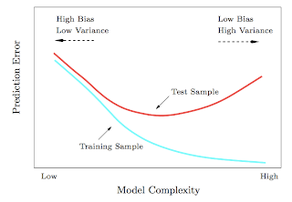
1. Test and training error: Why lower training error is not always a good thing: ESL Figure 2.11. Test and training error as a function of model complexity.

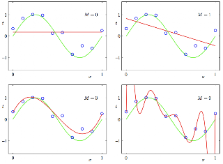
2. Under and overfitting: PRML Figure 1.4. Plots of polynomials having various orders M, shown as red curves, fitted to the data set generated by the green curve.

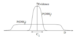
3. Occam's razor: ITILA Figure 28.3. Why Bayesian inference embodies Occam’s razor. This figure gives the basic intuition for why complex models can turn out to be less probable. The horizontal axis represents the space of possible data sets D. Bayes’ theorem rewards models in proportion to how much they predicted the data that occurred. These predictions are quantified by a normalized probability distribution on D. This probability of the data given model Hi, P (D | Hi), is called the evidence for Hi. A simple model H1 makes only a limited range of predictions, shown by P(D|H1); a more powerful model H2, that has, for example, more free parameters than H1, is able to predict a greater variety of data sets. This means, however, that H2 does not predict the data sets in region C1 as strongly as H1. Suppose that equal prior probabilities have been assigned to the two models. Then, if the data set falls in region C1, the less powerful model H1 will be the more probable model.

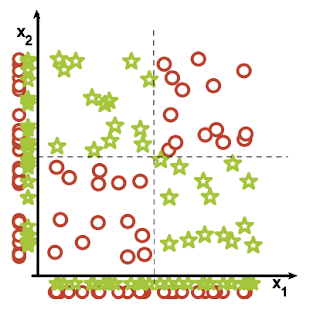
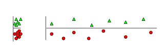
4. Feature combinations: (1) Why collectively relevant features may look individually irrelevant, and also (2) Why linear methods may fail. From Isabelle Guyon's feature extraction slides.

5. Irrelevant features: Why irrelevant features hurt kNN, clustering, and other similarity based methods. The figure on the left shows two classes well separated on the vertical axis. The figure on the right adds an irrelevant horizontal axis which destroys the grouping and makes many points nearest neighbors of the opposite class.

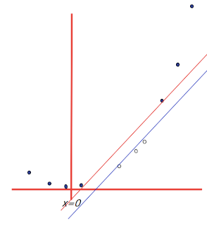
6. Basis functions: How non-linear basis functions turn a low dimensional classification problem without a linear boundary into a high dimensional problem with a linear boundary. From SVM tutorial slides by Andrew Moore: a one dimensional non-linear classification problem with input x is turned into a 2-D problem z=(x, x^2) that is linearly separable.

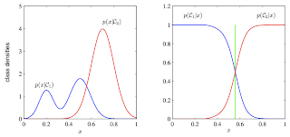
7. Discriminative vs. Generative: Why discriminative learning may be easier than generative: PRML Figure 1.27. Example of the class-conditional densities for two classes having a single input variable x (left plot) together with the corresponding posterior probabilities (right plot). Note that the left-hand mode of the class-conditional density p(x|C1), shown in blue on the left plot, has no effect on the posterior probabilities. The vertical green line in the right plot shows the decision boundary in x that gives the minimum misclassification rate.

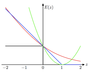
8. Loss functions: Learning algorithms can be viewed as optimizing different loss functions: PRML Figure 7.5. Plot of the ‘hinge’ error function used in support vector machines, shown in blue, along with the error function for logistic regression, rescaled by a factor of 1/ln(2) so that it passes through the point (0, 1), shown in red. Also shown are the misclassification error in black and the squared error in green.

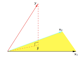
9. Geometry of least squares: ESL Figure 3.2. The N-dimensional geometry of least squares regression with two predictors. The outcome vector y is orthogonally projected onto the hyperplane spanned by the input vectors x1 and x2. The projection yˆ represents the vector of the least squares predictions.

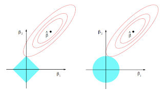
10. Sparsity: Why Lasso (L1 regularization or Laplacian prior) gives sparse solutions (i.e. weight vectors with more zeros): ESL Figure 3.11. Estimation picture for the lasso (left) and ridge regression (right). Shown are contours of the error and constraint functions. The solid blue areas are the constraint regions |β1| + |β2| ≤ t and β1² + β2² ≤ t2, respectively, while the red ellipses are the contours of the least squares error function.

from: http://www.denizyuret.com/2014/02/machine-learning-in-5-pictures.html