Numerical Analysis

PART1  <求解方程>

1，二分法

def bisect(f,a,b,TOL=0.000004):
    u_a = a
    u_b = b
    while(u_b-u_a)/2.0 > TOL:
        c = (u_a+u_b)/2.0
        if f(c) == :
            break
        if f(u_a)*f(c) < :
            u_b = c
        else:
            u_a = c

    u_c = (u_a + u_b) / 2.0
    return u_c

f = lambda x: x*x*x + x -
ret = bisect(f,-1.0,1.0)
print(ret)

print(f(ret))

2,不动点迭代法求解方程(FPI)

例如求cosx - x = 0 方程 事实上可以化成x = cosx

x^3 + x - 1 = 0 也可以化成 x=1 - x^3

等式左边是x 右边设为f(x)

即是:x = f(x)

过程如下:
x1 = f(x0)
x2 = f(x1)
x3 = f(x2)
........

例如求cosx = x  即(cosx -  x = 0）的解:  他的不动点是0.7390851332

def fpi(f,x0,k):
    xvalues = []
    xvalues.append(x0)
    for i in range(k):
        xvalues.append(f(xvalues[i]))
    print(xvalues)
    return xvalues[-1]  # return last

import math
f = lambda x:math.cos(x)
v = fpi(f,0,10)
print(v)

上述代码迭代十次 可以看到生成的数值为:

[0, 1.0, 0.5403023058681398, 0.8575532158463933, 0.6542897904977792, 0.7934803587425655, 0.7013687736227566, 
0.7639596829006542, 0.7221024250267077, 0.7504177617637605, 0.7314040424225098, 0.7442373549005569, 
0.7356047404363473, 0.7414250866101093, 0.7375068905132428, 0.7401473355678757, 0.7383692041223232, 
0.739567202212256, 0.7387603198742114, 0.7393038923969057, 0.7389377567153446]

20次基本达到了与精确解

PART2  <求解方程组>

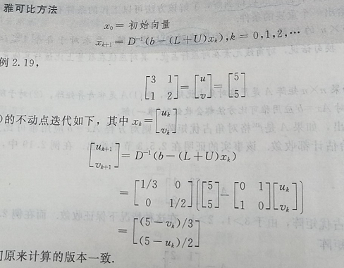
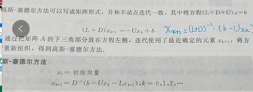
3，雅克比(jacobi)和高斯-赛德尔(Gauss-Seidel) 解方程组

结论:高斯-赛德尔的收敛速度比雅克比快的多。Gauss-Seidel20次迭代达到精确解，jacobi 20次还没得到

还有个高斯-赛德尔SOR 实现起来比较简单。

D代表对角阵，除了对角元素其他都为0

L,除了对角元素往下的元素，其他都为0

U,除了对角元素往上的元素，其他都为0

注意这里的LU和 LU分解是有本质的区别。

高斯赛的尔 用的我蓝色标识的字:

import numpy as np

class GMatrix:
    @staticmethod
    def Invert(matrix):
        nm = np.linalg.inv(matrix.mmatrix)
        gm = GMatrix()
        gm.assignNumPyMatrix(nm)
        return gm

    def __init__(self, nx=0, ny=0):
        self.rows = nx
        self.columns = ny
        self.mmatrix = np.matrix(np.zeros((nx, ny)))

    def assignNumPyMatrix(self, matrix):
        self.mmatrix = matrix

    def changeShape(self, nx, ny):
        self.mmatrix = np.matrix(np.zeros((nx, ny)))

    def debug(self):
        print("{\n", ">>SHAPE:", (self.mmatrix.shape))
        print(self.mmatrix)
        print('}\n')

    def numPyMatrix(self):
        return self.mmatrix

    def set(self, i, j, var):
        self.mmatrix[i - 1, j - 1] = var

    def get(self, i, j):
        return self.mmatrix[i - 1, j - 1]

    def L(self):
        n = self.rows
        m = GMatrix(n, n)

        for j in range(1, n, 1):
            for i in range(j + 1, n + 1):
                # print(i, j)
                m.set(i, j, self.get(i, j))
        return m

    def U(self):
        n = self.rows
        m = GMatrix(n, n)
        for i in range(1, n + 1, 1):
            for j in range(i + 1, n + 1):
                m.set(i, j, self.get(i, j))
        return m

    def D(self):
        """
        this matrix diagonal values
        1,make a empty matrix
        2,copy diagonal value to this empty matrix
        """
        n = self.rows
        m = GMatrix(n, n)
        for i in range(self.rows):
            index = i + 1
            m.set(index, index, self.get(index, index))
        return m

    def DInvert(self):
        """
        invert diagonal matrix !
        :return:
        """
        n = self.rows
        m = GMatrix(n, n)
        for i in range(n):
            index = i + 1
            m.set(index, index, 1 / self.get(index, index))
        return m

    def __mul__(self, other):
        nm = self.mmatrix * other.mmatrix  # USE NumPy matrix * matrix
        m = GMatrix()
        m.assignNumPyMatrix(nm)
        return m

    def __add__(self, other):
        nm = self.mmatrix + other.mmatrix  # USE NumPy matrix + matrix
        m = GMatrix()
        m.assignNumPyMatrix(nm)
        return m

    def __sub__(self, other):
        nm = self.mmatrix - other.mmatrix  # USE NumPy matrix - matrix
        m = GMatrix()
        m.assignNumPyMatrix(nm)
        return m

def Jacobi_Solver(x0, L, U, invertD, b,iter =20):
    """
    x0   = INIT_VECTOR_VALUE
    xk+1 = Inv(D)*[ b-(L+U)xk ]  ,k = 0,1,2,......
    :return:
    """
    nextX = x0
    for x in range(iter):
        nextX = invertD * (b - (L + U) * nextX)
    return nextX

def Gauss_Seidel_Solver(x0, L, U, D, b,iter =10):
    """
    xk+1 = inv(L+D) * (b- U*xk)

    """
    nextX = x0
    for x in range(iter):
        nextX = GMatrix.Invert(L+D) * (b - U * nextX)
    return nextX

def unit_test_matrix():
    m = GMatrix(2, 2)
    m.set(1, 1, 3)
    m.set(1, 2, 1)
    m.set(2, 1, 1)
    m.set(2, 2, 2)

    # and also can this
    # m.numPyMatrix()[0, 0] = 3
    # m.numPyMatrix()[0, 1] = 1
    # m.numPyMatrix()[1, 0] = 1
    # m.numPyMatrix()[1, 1] = 2
    m.debug()
    m.D().debug()
    m.L().debug()
    m.U().debug()
    m.DInvert().debug()

def unit_test_jacobi():
    """
    |  3 1  |   |u|      |5|
    |       |   | |   =  | |
    |  1 2  |   |v|      |5|

    --------
    AX = b
    --------
    :return:
    """

    # CONSTRUCT THE A MATRIX
    A = GMatrix(2, 2)
    A.set(1, 1, 3)  # A11 = 3
    A.set(1, 2, 1)  # A12 = 1
    A.set(2, 1, 1)  # A21 = 1
    A.set(2, 2, 2)  # A22 = 2
    #A.debug()

    # CONSTRUCT THE b vector
    b = GMatrix(2, 1)
    b.set(1, 1, 5)
    b.set(2, 1, 5)

    # INIT zero vector to iter
    x0 = GMatrix(2,1) # [0,0]T vector initialize

    invert_D = A.DInvert()

    L = A.L()
    U = A.U()

    print("get the jacobi result ")
    Jacobi_Solver(x0,L,U,invert_D,b).debug()

def unit_test_Gauss_Seidel():
    """
        |  3 1  |   |u|      |5|
        |       |   | |   =  | |
        |  1 2  |   |v|      |5|

        --------
        AX = b
        --------
        :return:
        """

    # CONSTRUCT THE A MATRIX
    A = GMatrix(2, 2)
    A.set(1, 1, 3)  # A11 = 3
    A.set(1, 2, 1)  # A12 = 1
    A.set(2, 1, 1)  # A21 = 1
    A.set(2, 2, 2)  # A22 = 2

    # CONSTRUCT THE b vector
    b = GMatrix(2, 1)
    b.set(1, 1, 5)
    b.set(2, 1, 5)

    # INIT zero vector to iter
    x0 = GMatrix(2, 1)  # [0,0]T vector initialize

    D = A.D()
    L = A.L()
    U = A.U()

    print("get the Gauss_Seidel result ")
    Gauss_Seidel_Solver(x0, L, U, D, b).debug()

unit_test_jacobi()
unit_test_Gauss_Seidel()

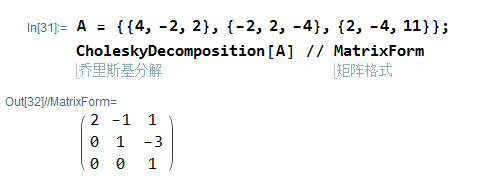
4,楚列斯基分解choleskyDecomposition

这类情况只适合于正定矩阵。

楚列斯基分解的目的就是将正定矩阵分解成A = transpose(R) * R .

求解方程组直接使用回代法即可求出向量解,

这类方法不是迭代法，最重要的是分解矩阵.

所以是要求出来这个上三角矩阵R,比如分解如下矩阵：

[[  4.  -2.   2.]
 [ -2.   2.  -4.]
 [  2.  -4.  11.]]

import numpy as np
import math

class GMatrix:
    def __init__(self, shape):
        self.nn = shape
        self.Mat = np.zeros((shape, shape))

    def setRawData(self, *args):
        if len(args) != self.nn * self.nn:
            raise ValueError

        deserialize = []
        for i in range(self.nn):
            rhtmp = []
            for j in range(self.nn):
                rhtmp.append(args[i * self.nn + j])
            deserialize.append(rhtmp)
        self.tupleToMatrix(deserialize)

    def tupleToMatrix(self, tupleObj):
        """
        :param tupleObj: ([1,2],[3,4])
        will set matrix above tuple obj
        """
        for i in range(self.nn):
            # get row data of args
            row_data = tupleObj[i]
            for j in range(self.nn):
                self.Mat[i, j] = row_data[j]

    def setRowsData(self, *args):
        if len(args) != self.nn:
            raise ValueError
        self.tupleToMatrix(args)

    def __str__(self):
        return str(self.Mat)

    def divideConstant(self, var):
        self.Mat[:, :] = self.Mat[:, :] / var

    def __add__(self, other):
        self.Mat[:, :] = self.Mat[:, :] + other.mat[:, :]

    def __sub__(self, other):
        self.Mat[:, :] = self.Mat[:, :] - other.mat[:, :]

    def nextLayer(self):
        array = self.Mat[1:, 1:]
        m = GMatrix(a.Mat.shape[0])
        m.Mat = array
        return m

    def getupu(self):
        self.Mat = np.triu(self.Mat)
        return self

def choleskyDecomposition(op=GMatrix(2)):
    """ DEFINE MATRIX:
    R11 R12 ... R1n
    R21 R22 ... R2n
     .   .       .
     .   .       .
    Rn1 Rn2 ... Rnn

    """
    if len(op.Mat.flatten()) == 1:
        op.Mat[op.nn - 1:, op.nn - 1:] = np.sqrt(op.Mat[op.nn - 1:, op.nn - 1:])
        return

    # First make the matrix A11 to sqrt(A11)
    op.Mat[0, 0] = math.sqrt(op.Mat[0, 0])  # R11
    op.Mat[0, 1:] = op.Mat[0, 1:] / op.Mat[0,0]  # (R12 R13 .... R1n) = (R12 R13 ...R1n) / R11

    # cal u.transpose(u)
    u   = np.matrix(op.Mat[0,1:])      # it's a row vector
    ut  = np.transpose(u)              # it's a column vector

    uut = ut*u
    # extract_layer - uut
    op.Mat[1:,1:] = op.Mat[1:,1:] - uut
    choleskyDecomposition(op.nextLayer())

a = GMatrix(3)

a.setRawData(4, -2, 2, -2, 2, -4, 2, -4, 11)
print(a)
choleskyDecomposition(a)
print(a.getupu())

分解结果R:

[[ 2. -1.  1.]
 [ 0.  1. -3.]
 [ 0.  0.  1.]]

Mathematica 检查结果:

5,共轭梯度法:

6,预条件共轭梯度法:

BVP:

差分法比较简单略.

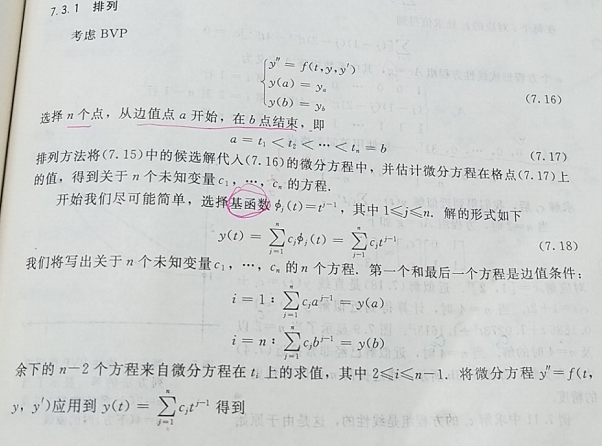
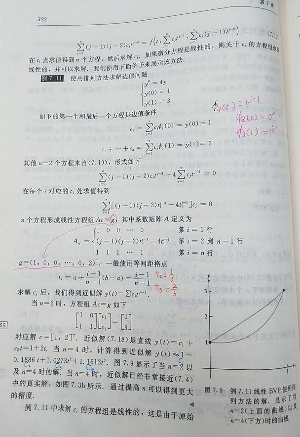
排列法求解BVP问题:

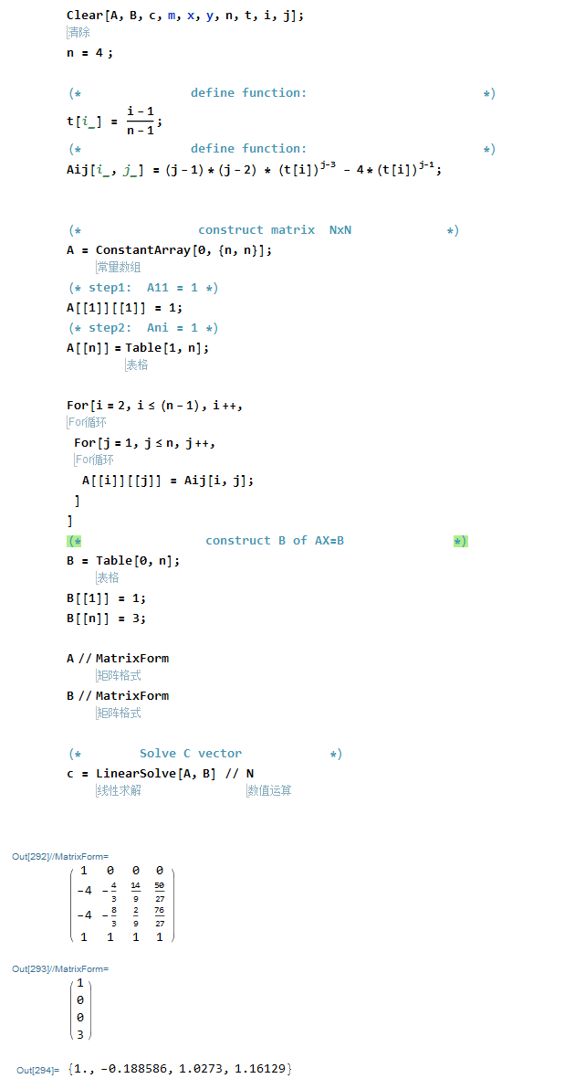
如下例，n=2书中已经给答案，n=4的矩阵未给出，顺便自己解下矩阵n=4的情况。

算出c1,c2,c3,c4:

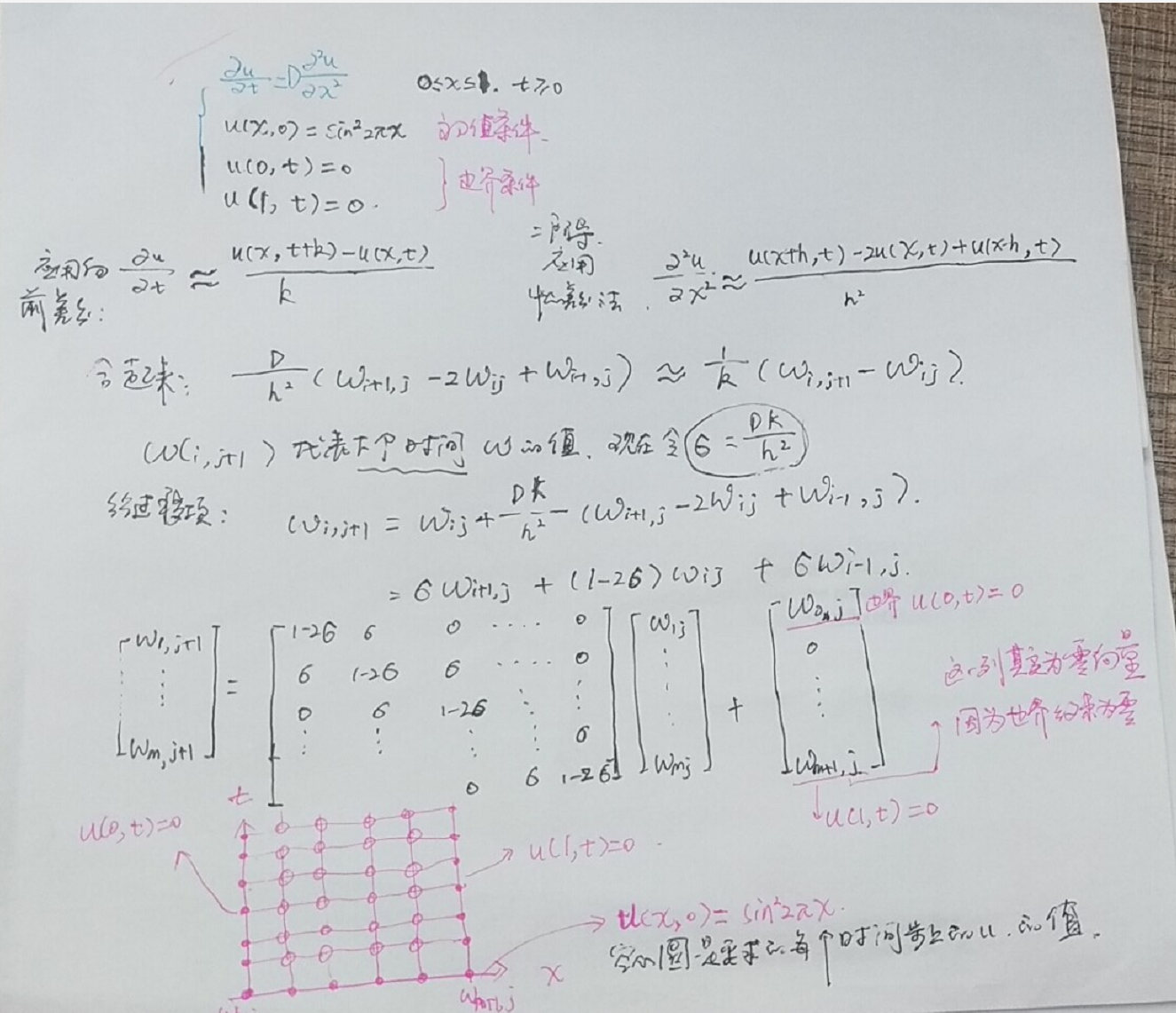
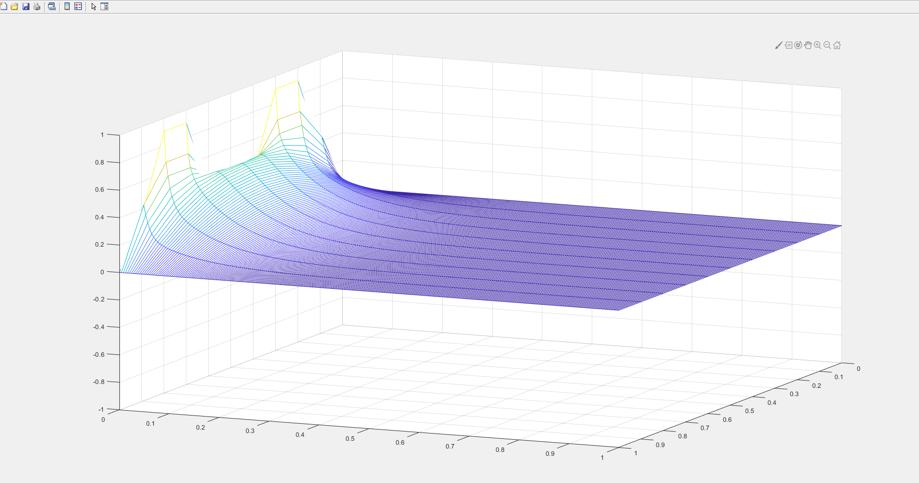
PDE 解热方程:

这次将时间方向放入坐标轴，可以用三维图像直接看到 在时间步上，热方程是如何传递的.

clc;
clear w a b c d M N f l r m sigma ;
xl = 0;
xr = 1;
yb = 0;
yt = 1;

M = 10;
N = 250;

f = @(x) sin(2*pi*x).^2;
l = @(t) 0*t;
r = @(t) 0*t;

D =1;
h = (xr-xl) / M
k = (yt-yb) / N
m = M -1;
n=N;
sigma = D*k/(h*h);

lside = l(yb+(0:n)*k);
rside = r(yb+(0:n)*k);

% 定义矩阵a
a = diag(1-2*sigma*ones(m,1));
a = a + diag(sigma*ones(m-1,1),1);  %自身加上  往右offset 1列 sigma倍数
a = a + diag(sigma*ones(m-1,1),-1); %自身加上  往左偏移 1列sigma倍数
a

% 设置w第一列 ,初值条件,注意 要转置，因为 设置 w的第一列向量
w(:,1) = f(xl + (1:m) * h)'

disp('START FOR LOOP')
% 给w 在时间250 迭代成列向量，则w是251列向量
for j = 1:n
    rhs = w(:,1)';
    w(:,j+1) = a*w(:,j) ;
end
disp('END FOR LOOP')

w = [lside;w;rside];
x = (0:m+1)*h; t= (0:n)*k;
mesh(x,t,w')
view(60,30);
axis([xl xr yb yt -1 1]);