DeepHyperX代码理解-HamidaEtAl

代码复现自论文《3-D Deep Learning Approach for Remote Sensing Image Classification》

先对部分基础知识做一些整理：

一、局部连接与参数共享（都减少了参数计算量）

　　局部连接：基于图像局部相关的原理，保留了图像局部结构，同时减少了网络的权值个数，加快了学习速率，同时也在一定程度上减少了过拟合的可能。

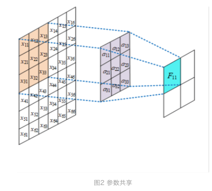
　　参数共享：下面用图例解释参数共享与不共享的区别。　　

　　如图是一个3*3大小的卷积核在进行特征提取，channel=1, 在每个位置进行特征提取的时候都是共享一个卷积核，假设有k个channel,则参数

总量为3*3*k,注意不同channel的参数是不能共享的。

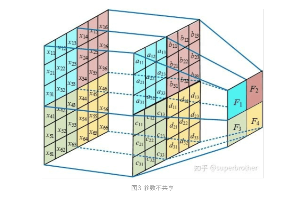
　　假设现在不使用参数共享，则卷积核作用于矩阵上的每一个位置时其参数都是不一样的，则卷积核的参数数量就与像素矩阵的大小保持一致了，假
设有k个channel,则参数数量为weight*height*k，这对于尺寸较大的图片来说明显是不可取的。

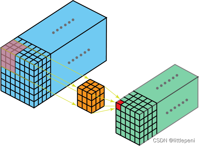
二、多通道输入输出：

　　首先理解fliter与kernel区别：kernel是fliter的组成成分，一个fliter就会对应生成一个特征图。

　　下图为多通道输入，单通道输出。有一个fliter，一个fliter包括三个kernel，最后生成一个特征图（一个fliter就对应一个特征图）

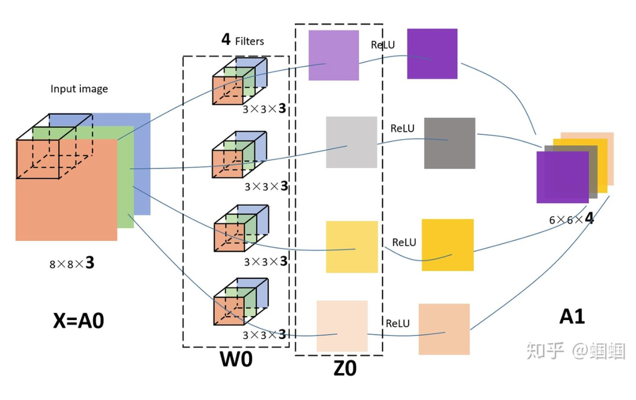
　　下图为直观展示，输入为8*8*3的RGB三通道图片，设置了4个fliter对应四个输出通道，也就是输出4个特征图。每个fliter有3个kernel。

三、2D卷积代码示例：

 1 import torch as t
 2 import torch.nn as nn
 3
 4 class A(nn.Module):
 5     def __init__(self):
 6         super(A, self).__init__()
 7         #三个2D卷积层结构，每个卷积层的输入和输出通道数均为2，卷积核和大小是(3, 3)
 8         #torch.nn.Conv2d(in_channels, out_channels, kernel_size, stride=1,
 9         #padding=0, dilation=1, groups=1, bias=True,
10         #padding_mode='zeros', device=None, dtype=None)
11         self.conv1 = nn.Conv2d(2, 2, kernel_size=(3, 3))
12         self.conv2 = nn.Conv2d(2, 2, kernel_size=(3, 3))
13         self.conv3 = nn.Conv2d(2, 2, kernel_size=(3, 3))
14
15 a = A()
16 print(list(a.parameters()))

运行结果：

 1 [Parameter containing:
 2 tensor([[[[ 0.0213, -0.2054,  0.0985],
 3           [ 0.1254,  0.1202, -0.1115],
 4           [-0.0280,  0.0256,  0.1975]],
 5
 6          [[-0.2118, -0.1683,  0.0056],
 7           [-0.0554,  0.2255, -0.1548],
 8           [ 0.1747,  0.0449,  0.1606]]],
 9
10
11         [[[-0.1328, -0.1700, -0.1048],
12           [ 0.0911, -0.2230,  0.0685],
13           [ 0.0886,  0.1765, -0.1879]],
14
15          [[-0.0581,  0.1266, -0.1030],
16           [-0.0170,  0.0387, -0.0641],
17           [-0.0127, -0.2099, -0.2213]]]], requires_grad=True), Parameter containing:
18 tensor([ 0.0877, -0.1969], requires_grad=True), Parameter containing:
19 tensor([[[[-0.0266,  0.1511, -0.0034],
20           [-0.1070, -0.1734, -0.1017],
21           [ 0.0053,  0.1358, -0.0542]],
22
23          [[-0.0436,  0.1587, -0.0375],
24           [ 0.0125, -0.0431, -0.0877],
25           [-0.0766,  0.0405, -0.1306]]],
26
27
28         [[[-0.1449, -0.0315, -0.0236],
29           [ 0.0118,  0.2230, -0.2137],
30           [-0.1108, -0.1178,  0.0027]],
31
32          [[ 0.2184,  0.1964, -0.0959],
33           [-0.0385, -0.0523,  0.2135],
34           [-0.0387,  0.1951, -0.1546]]]], requires_grad=True), Parameter containing:
35 tensor([-0.0942, -0.2029], requires_grad=True), Parameter containing:
36 tensor([[[[ 8.9598e-02, -3.3190e-02,  1.0606e-01],
37           [-2.2397e-02,  2.0944e-01, -6.8180e-02],
38           [-1.7312e-01,  2.2318e-01,  1.9368e-01]],
39
40          [[ 7.0529e-02, -2.0741e-01, -1.2648e-01],
41           [-1.7503e-01,  1.7972e-01, -1.0417e-01],
42           [-1.9124e-01, -4.2022e-02,  1.4635e-01]]],
43
44
45         [[[-8.0857e-02,  8.5098e-03,  7.0629e-02],
46           [ 1.6926e-01, -1.7654e-02, -9.3033e-02],
47           [-2.9836e-02, -2.2935e-01,  1.1450e-01]],
48
49          [[ 1.3848e-01, -5.7713e-02,  1.5293e-04],
50           [-6.3998e-03, -1.0745e-01,  2.8835e-03],
51           [-1.7894e-01,  2.2133e-01,  5.2435e-02]]]], requires_grad=True), Parameter containing:
52 tensor([-0.1026,  0.0207], requires_grad=True)]

　　上面代码是定义的一个2D卷积网络架构，有3个卷积层，每个卷积层的输入通道和输出通道（对应fliter为2）都为2，每个fliter中有两个3*3的kernel（对应两个输入通道）。代码中的两个1*2的向量为bias。

四、3D卷积的示意图和示例代码：

 1 class B(nn.Module):
 2     def __init__(self):
 3         super(B, self).__init__()
 4         self.conv1 = nn.Conv3d(
 5             1,  # 输入图像的channel数,C_in
 6             3,  # 卷积产生的channel数,C_out
 7             kernel_size=2,  # 卷积核的尺寸,这里实际是(2,2,2),第一维表示卷积核处理的帧数
 8             stride=(1,1,1),  # 卷积步长,(D,H,W)
 9             padding=(0,0,0),  # 输入的每一条边补充0的层数,(D,H,W)
10             bias=False)
11         self.conv2 = nn.Conv3d(1, 3, kernel_size=(2, 2, 2), stride=(1, 1, 1), padding=(0, 0, 0), bias=False)
12
13 b = B()
14 print(list(b.parameters()))

运行结果：

 1 [Parameter containing:
 2 tensor([[[[[-0.0895, -0.1651],
 3            [-0.1319,  0.2510]],
 4
 5           [[-0.1616, -0.2614],
 6            [ 0.0383,  0.2656]]]],
 7
 8
 9
10         [[[[-0.0809, -0.1821],
11            [-0.0624, -0.1401]],
12
13           [[-0.3170,  0.1499],
14            [-0.3449,  0.2639]]]],
15
16
17
18         [[[[ 0.2779, -0.0731],
19            [ 0.0439, -0.0353]],
20
21           [[ 0.2853, -0.3177],
22            [ 0.0559, -0.3290]]]]], requires_grad=True), Parameter containing:
23 tensor([[[[[-0.2529, -0.0537],
24            [ 0.0955, -0.1513]],
25
26           [[ 0.0310,  0.2558],
27            [-0.1903, -0.1561]]]],
28
29
30
31         [[[[-0.2919, -0.3142],
32            [ 0.0190, -0.1089]],
33
34           [[-0.0586,  0.1541],
35            [-0.2402, -0.3339]]]],
36
37
38
39         [[[[-0.3260, -0.0500],
40            [ 0.1392,  0.1486]],
41
42           [[ 0.1664,  0.1514],
43            [ 0.0345, -0.1979]]]]], requires_grad=True)]

　　三维数据输入通道为1，输出通道为3，那么fliter数为3，每个fliter中有1个kernel(2,2,2),因为两个3Dconv参数一样，所以每个3Dconv有3个2*2*2的tensor。这里如果对应到高光谱数据集，输入通道也为1。因为整个高光谱数据集就是一个3维的volume，整个数据集图像由长*宽*光谱维组成。

论文复现：

原论文网络结构:

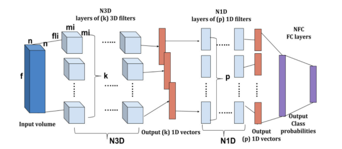
复现网络：

输入维度：Image has dimensions 610x340 and 103 channels

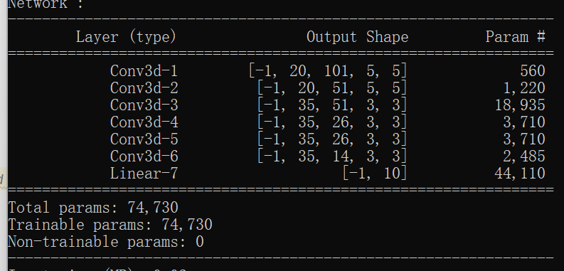
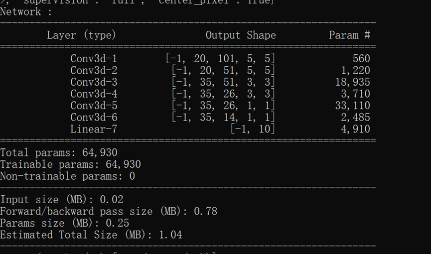
网络结构及参数：

 复现代码：

1     elif name == "hamida":
2         patch_size = kwargs.setdefault("patch_size", 5)
3         center_pixel = True
4         model = HamidaEtAl(n_bands, n_classes, patch_size=patch_size)
5         lr = kwargs.setdefault("learning_rate", 0.01)
6         optimizer = optim.SGD(model.parameters(), lr=lr, weight_decay=0.0005)
7         kwargs.setdefault("batch_size", 100)
8         criterion = nn.CrossEntropyLoss(weight=kwargs["weights"])

 1 class HamidaEtAl(nn.Module):
 2     """
 3     3-D Deep Learning Approach for Remote Sensing Image Classification
 4     Amina Ben Hamida, Alexandre Benoit, Patrick Lambert, Chokri Ben Amar
 5     IEEE TGRS, 2018
 6     https://ieeexplore.ieee.org/stamp/stamp.jsp?arnumber=8344565
 7     """
 8
 9     @staticmethod
10     def weight_init(m):#权重初始化
11         if isinstance(m, nn.Linear) or isinstance(m, nn.Conv3d):
12             init.kaiming_normal_(m.weight) #kaiming_normal_均匀初始化方法
13             init.zeros_(m.bias)
14
15     def __init__(self, input_channels, n_classes, patch_size=5, dilation=1):
16         super(HamidaEtAl, self).__init__()
17         # The first layer is a (3,3,3) kernel sized Conv characterized
18         # by a stride equal to 1 and number of neurons equal to 20
19         self.patch_size = patch_size#每次截取图像patch大小(5,5)
20         self.input_channels = input_channels#输入通道数（波段数）
21         dilation = (dilation, 1, 1)
22
23         if patch_size == 3:
24             self.conv1 = nn.Conv3d(
25                 1, 20, (3, 3, 3), stride=(1, 1, 1), dilation=dilation, padding=1
26             )
27         else:
28             self.conv1 = nn.Conv3d(
29                 1, 20, (3, 3, 3), stride=(1, 1, 1), dilation=dilation, padding=0
30             )
31         # Next pooling is applied using a layer identical to the previous one
32         # with the difference of a 1D kernel size (1,1,3) and a larger stride
33         # equal to 2 in order to reduce the spectral dimension
34         #为什么要用卷积层要替代池化层：
35         # 使用2×2的最大池化，与使用卷积（stride为2）来做down sample性能并没有明显差别，
36         # 而且使用卷积（stride为2）相比卷积（步进为1）+池化，还可以减少卷积运算量和一个池化层。何乐而不为呢。
37         self.pool1 = nn.Conv3d(
38             20, 20, (3, 1, 1), dilation=dilation, stride=(2, 1, 1), padding=(1, 0, 0)
39         )
40         # Then, a duplicate of the first and second layers is created with
41         # 35 hidden neurons per layer.
42         self.conv2 = nn.Conv3d(
43             20, 35, (3, 3, 3), dilation=dilation, stride=(1, 1, 1), padding=(1, 0, 0)
44         )
45         self.pool2 = nn.Conv3d(
46             35, 35, (3, 1, 1), dilation=dilation, stride=(2, 1, 1), padding=(1, 0, 0)
47         )
48         # Finally, the 1D spatial dimension is progressively reduced
49         # thanks to the use of two Conv layers, 35 neurons each,
50         # with respective kernel sizes of (1,1,3) and (1,1,2) and strides
51         # respectively equal to (1,1,1) and (1,1,2)
52         self.conv3 = nn.Conv3d(
53             35, 35, (3, 1, 1), dilation=dilation, stride=(1, 1, 1), padding=(1, 0, 0)
54         )
55         self.conv4 = nn.Conv3d(
56             35, 35, (2, 1, 1), dilation=dilation, stride=(2, 1, 1), padding=(1, 0, 0)
57         )
58
59         # self.dropout = nn.Dropout(p=0.5)
60
61         self.features_size = self._get_final_flattened_size()
62         # The architecture ends with a fully connected layer where the number
63         # of neurons is equal to the number of input classes.
64         self.fc = nn.Linear(self.features_size, n_classes)
65
66         self.apply(self.weight_init)
67
68     def _get_final_flattened_size(self):#计算fc前的输出tensor大小，用随机的X去测试得到，这样就不用自己去推到了
69         with torch.no_grad():
70             x = torch.zeros(
71                 (1, 1, self.input_channels, self.patch_size, self.patch_size)
72             )
73             x = self.pool1(self.conv1(x))
74             x = self.pool2(self.conv2(x))
75             x = self.conv3(x)
76             x = self.conv4(x)
77             _, t, c, w, h = x.size()
78         return t * c * w * h
79
80     def forward(self, x):
81         x = F.relu(self.conv1(x))
82         x = self.pool1(x)
83         x = F.relu(self.conv2(x))
84         x = self.pool2(x)
85         x = F.relu(self.conv3(x))
86         x = F.relu(self.conv4(x))
87         x = x.view(-1, self.features_size)#对tensor resize相当于做展平（flatten）操作
88         # x = self.dropout(x)
89         x = self.fc(x)
90         return x

关于参数dilation的解释：https://blog.csdn.net/qimo601/article/details/112624091

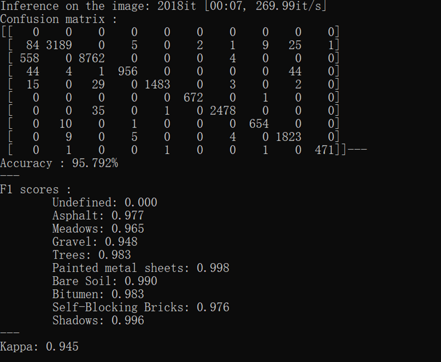
运行结果：

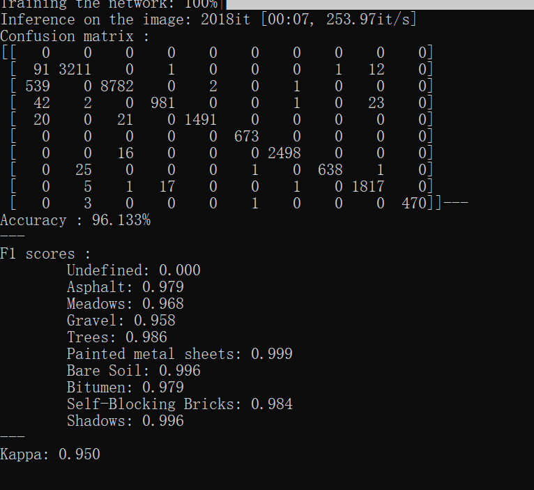
通过阅读代码发现和原论文中的结构并不完全相同，试着去修改了一层网络参数去接近原网络结构：

self.conv3 = nn.Conv3d(
            35, 35, (3, 1, 1), dilation=dilation, stride=(1, 1, 1), padding=(1, 0, 0)
        )

->>

self.conv3 = nn.Conv3d(
            35, 35, (3, 3, 3), dilation=dilation, stride=(1, 1, 1), padding=(1, 0, 0)
        )

但发现最终效果不如上面结果，可能是对原论文提出的结构稍作改进了吧。

参考资料：

https://github.com/nshaud/DeepHyperX

https://blog.csdn.net/weixin_38481963/article/details/109906338

https://blog.csdn.net/abbcdc/article/details/123332063

https://wenku.baidu.com/view/fa899796f221dd36a32d7375a417866fb84ac087.html