python数字图像处理（三）边缘检测常用算子

在该文将介绍基本的几种应用于边缘检测的滤波器,首先我们读入saber用来做为示例的图像

#读入图像代码,在此之前应当引入必要的opencv matplotlib numpy
saber = cv2.imread("saber.png")
saber = cv2.cvtColor(saber,cv2.COLOR_BGR2RGB)
plt.imshow(saber)
plt.axis("off")
plt.show()

使用上图作为滤波器使用的图形

Roberts 交叉梯度算子

Roberts交叉梯度算子由两个\(2\times2\)的模版构成，如图。

\[ \begin{bmatrix}
-1 & 0 \\
0 & 1
\end{bmatrix}
\]

\[ \begin{bmatrix}
0 & -1 \\
1 & 0
\end{bmatrix}
\]

对如图的矩阵分别才用两个模版相乘，并加在一起

\[ \begin{bmatrix}
Z_1 & Z_2 & Z_3 \\
Z_4 & Z_5 & Z_6 \\
Z_7 & Z_8 & Z_9 \\
\end{bmatrix}
\]

简单表示即

\(|z_9-z_5|+|z_8-z_6|\)。

可以简单用编程实现

首先将原图像进行边界扩展，并将其转换为灰度图。

gray_saber = cv2.cvtColor(saber,cv2.COLOR_RGB2GRAY)
gray_saber = cv2.resize(gray_saber,(200,200))

在接下来的的代码中我们对图像都会进行边界扩展，是因为将图像增加宽度为1的图像能够使在计算3*3的算子时不用考虑边界情况

def RobertsOperator(roi):
    operator_first = np.array([[-1,0],[0,1]])
    operator_second = np.array([[0,-1],[1,0]])
    return np.abs(np.sum(roi[1:,1:]*operator_first))+np.abs(np.sum(roi[1:,1:]*operator_second))
def RobertsAlogrithm(image):
    image = cv2.copyMakeBorder(image,1,1,1,1,cv2.BORDER_DEFAULT)
    for i in range(1,image.shape[0]):
        for j in range(1,image.shape[1]):
            image[i,j] = RobertsOperator(image[i-1:i+2,j-1:j+2])
    return image[1:image.shape[0],1:image.shape[1]]

Robert_saber = RobertsAlogrithm(gray_saber)

plt.imshow(Robert_saber,cmap="binary")
plt.axis("off")
plt.show()

python的在这种纯计算方面实在有些慢，当然这也是因为我过多的使用了for循环而没有利用好numpy的原因

我们可以看出Roberts算子在检测边缘效果已经相当不错了，但是它对噪声相当敏感，我们给它加上噪声在看看它的效果

噪声代码来源于stacksoverflow

def noisy(noise_typ,image):
    if noise_typ == "gauss":
        row,col,ch= image.shape
        mean = 0
        var = 0.1
        sigma = var**0.5
        gauss = np.random.normal(mean,sigma,(row,col,ch))
        gauss = gauss.reshape(row,col,ch)
        noisy = image + gauss
        return noisy
    elif noise_typ == "s&p":
        row,col,ch = image.shape
        s_vs_p = 0.5
        amount = 0.004
        out = np.copy(image)
        num_salt = np.ceil(amount * image.size * s_vs_p)
        coords = [np.random.randint(0, i - 1, int(num_salt))
              for i in image.shape]
        out[coords] = 1
        num_pepper = np.ceil(amount* image.size * (1. - s_vs_p))
        coords = [np.random.randint(0, i - 1, int(num_pepper)) for i in image.shape]
        out[coords] = 0
        return out
    elif noise_typ == "poisson":
        vals = len(np.unique(image))
        vals = 2 ** np.ceil(np.log2(vals))
        noisy = np.random.poisson(image * vals) / float(vals)
        return noisy
    elif noise_typ =="speckle":
        row,col,ch = image.shape
        gauss = np.random.randn(row,col,ch)
        gauss = gauss.reshape(row,col,ch)
        noisy = image + image * gauss
        return noisy

dst = noisy("s&p",saber)
plt.subplot(121)
plt.title("add noise")
plt.axis("off")
plt.imshow(dst)
plt.subplot(122)
dst = cv2.cvtColor(dst,cv2.COLOR_RGB2GRAY)
plt.title("Robert Process")
plt.axis("off")
dst = RobertsAlogrithm(dst)
plt.imshow(dst,cmap="binary")
plt.show()

这里我们可以看出Robert算子对于噪声过于敏感,在加了噪声后,人的边缘变得非常不清晰

Prewitt算子

Prewitt算子是一种\(3\times3\)模板的算子,它有两种形式,分别表示水平和垂直的梯度.

垂直梯度

\[ \begin{bmatrix}
-1 & -1 & -1 \\
0 & 0 & 0 \\
1 & 1 & 1 \\
\end{bmatrix}
\]

水平梯度

\[ \begin{bmatrix}
-1 & 0 & 1 \\
-1 & 0 & 1 \\
-1 & 0 & 1 \\
\end{bmatrix}
\]

对于如图的矩阵起始值

\[ \begin{bmatrix}
Z_1 & Z_2 & Z_3 \\
Z_4 & Z_5 & Z_6 \\
Z_7 & Z_8 & Z_9 \\
\end{bmatrix}
\]

就是以下两个式子

\[|(z_7+z_8+z_9)-(z_1+z_2+z_3)|
\]

\[|(z_1+z_4+z_7)-(z_3+z_6+z_9)|
\]

1与-1更换位置对结果并不会产生影响

def PreWittOperator(roi,operator_type):
    if operator_type == "horizontal":
        prewitt_operator = np.array([[-1,-1,-1],[0,0,0],[1,1,1]])
    elif operator_type == "vertical":
        prewitt_operator = np.array([[-1,0,1],[-1,0,1],[-1,0,1]])
    else:
        raise("type Error")
    result = np.abs(np.sum(roi*prewitt_operator))
    return result

def PreWittAlogrithm(image,operator_type):
    new_image = np.zeros(image.shape)
    image = cv2.copyMakeBorder(image,1,1,1,1,cv2.BORDER_DEFAULT)
    for i in range(1,image.shape[0]-1):
        for j in range(1,image.shape[1]-1):
            new_image[i-1,j-1] = PreWittOperator(image[i-1:i+2,j-1:j+2],operator_type)
    new_image = new_image*(255/np.max(image))
    return new_image.astype(np.uint8)

在PreWitt算子执行中要考虑大于255的情况,使用下面代码

    new_image = new_image*(255/np.max(image))

将其放缩到0-255之间,并使用astype将其转换到uint8类型

plt.subplot(121)
plt.title("horizontal")
plt.imshow(PreWittAlogrithm(gray_saber,"horizontal"),cmap="binary")
plt.axis("off")
plt.subplot(122)
plt.title("vertical")
plt.imshow(PreWittAlogrithm(gray_saber,"vertical"),cmap="binary")
plt.axis("off")
plt.show()

现在我们看一下Prewitt对噪声的敏感性

dst = noisy("s&p",saber)
plt.subplot(131)
plt.title("add noise")
plt.axis("off")
plt.imshow(dst)

plt.subplot(132)
plt.title("Prewitt Process horizontal")
plt.axis("off")
plt.imshow(PreWittAlogrithm(gray_saber,"horizontal"),cmap="binary")

plt.subplot(133)
plt.title("Prewitt Process vertical")
plt.axis("off")
plt.imshow(PreWittAlogrithm(gray_saber,"vertical"),cmap="binary")
plt.show()

选择水平梯度或垂直梯度从上图可以看出对于边缘的影响还是相当大的.

Sobel算子

Sobel算子根据像素点上下、左右邻点灰度加权差，在边缘处达到极值这一现象检测边缘。对噪声具有平滑作用，提供较为精确的边缘方向信息，边缘定位精度不够高。当对精度要求不是很高时，是一种较为常用的边缘检测方法。相比Prewitt他周边像素对于判断边缘的贡献是不同的.

垂直梯度

\[ \begin{bmatrix}
-1 & -2 & -1 \\
0 & 0 & 0 \\
1 & 2 & 1 \\
\end{bmatrix}
\]

水平梯度

\[ \begin{bmatrix}
-1 & 0 & 1 \\
-2 & 0 & 2 \\
-1 & 0 & 1 \\
\end{bmatrix}
\]

对上面的代码稍微修改算子即可

def SobelOperator(roi,operator_type):
    if operator_type == "horizontal":
        sobel_operator = np.array([[-1,-2,-1],[0,0,0],[1,2,1]])
    elif operator_type == "vertical":
        sobel_operator = np.array([[-1,0,1],[-2,0,2],[-1,0,1]])
    else:
        raise("type Error")
    result = np.abs(np.sum(roi*sobel_operator))
    return result

def SobelAlogrithm(image,operator_type):
    new_image = np.zeros(image.shape)
    image = cv2.copyMakeBorder(image,1,1,1,1,cv2.BORDER_DEFAULT)
    for i in range(1,image.shape[0]-1):
        for j in range(1,image.shape[1]-1):
            new_image[i-1,j-1] = SobelOperator(image[i-1:i+2,j-1:j+2],operator_type)
    new_image = new_image*(255/np.max(image))
    return new_image.astype(np.uint8)

plt.subplot(121)
plt.title("horizontal")
plt.imshow(SobelAlogrithm(gray_saber,"horizontal"),cmap="binary")
plt.axis("off")
plt.subplot(122)
plt.title("vertical")
plt.imshow(SobelAlogrithm(gray_saber,"vertical"),cmap="binary")
plt.axis("off")
plt.show()

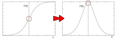
无论是Sobel还是Prewitt其实是求了单个方向颜色变化的极值

在某个方向上颜色的变化如图(此图来源于opencv官方文档)

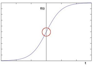
对其求导可以得到这样一条曲线

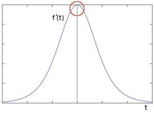
由此我们可以得知边缘可以通过定位梯度值大于邻域的相素的方法找到(或者推广到大于一个阀值).

而Sobel就是利用了这一定理

Laplace算子

无论是Sobel还是Prewitt都是求单方向上颜色变化的一阶导(Sobel相比Prewitt增加了权重),那么如何才能反映空间上的颜色变化的一个极值呢?



我们试着在对边缘求一次导



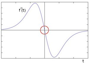
在一阶导数的极值位置，二阶导数为0。所以我们也可以用这个特点来作为检测图像边缘的方法。 但是， 二阶导数的0值不仅仅出现在边缘(它们也可能出现在无意义的位置),但是我们可以过滤掉这些点。

在实际情况中我们不可能用0作为判断条件,而是设定一个阈值,这就引出来Laplace算子

\begin{bmatrix}

0 & 1 & 0 \

1 & -4 & 1 \

0 & 1 & 0 \

\end{bmatrix}

\begin{bmatrix}

1 & 1 & 1 \

1 & -8 & 1 \

1 & 1 & 1 \

\end{bmatrix}

def LaplaceOperator(roi,operator_type):
    if operator_type == "fourfields":
        laplace_operator = np.array([[0,1,0],[1,-4,1],[0,1,0]])
    elif operator_type == "eightfields":
        laplace_operator = np.array([[1,1,1],[1,-8,1],[1,1,1]])
    else:
        raise("type Error")
    result = np.abs(np.sum(roi*laplace_operator))
    return result

def LaplaceAlogrithm(image,operator_type):
    new_image = np.zeros(image.shape)
    image = cv2.copyMakeBorder(image,1,1,1,1,cv2.BORDER_DEFAULT)
    for i in range(1,image.shape[0]-1):
        for j in range(1,image.shape[1]-1):
            new_image[i-1,j-1] = LaplaceOperator(image[i-1:i+2,j-1:j+2],operator_type)
    new_image = new_image*(255/np.max(image))
    return new_image.astype(np.uint8)

plt.subplot(121)
plt.title("fourfields")
plt.imshow(LaplaceAlogrithm(gray_saber,"fourfields"),cmap="binary")
plt.axis("off")
plt.subplot(122)
plt.title("eightfields")
plt.imshow(LaplaceAlogrithm(gray_saber,"eightfields"),cmap="binary")
plt.axis("off")
plt.show()

上图为比较取值不同的laplace算子实现的区别.

Canny算子

Canny边缘检测算子是一种多级检测算法。1986年由John F. Canny提出，同时提出了边缘检测的三大准则：

• 低错误率的边缘检测：检测算法应该精确地找到图像中的尽可能多的边缘，尽可能的减少漏检和误检。
• 最优定位：检测的边缘点应该精确地定位于边缘的中心。
• 图像中的任意边缘应该只被标记一次，同时图像噪声不应产生伪边缘。

Canny边缘检测算法的实现较为复杂,主要分为以下步骤,

1. 高斯模糊
2. 计算梯度幅值和方向
3. 非极大值 抑制
4. 滞后阈值

高斯模糊

在前面的章节中已经实现过均值模糊,模糊在图像处理中经常用来去除一些无关的细节.

均值模糊引出了另一个思考,周边每个像素点的权重设为一样是否合适?

(周边像素点的权重是很多算法的区别,比如Sobel和Prewitt)

因此概率中非常熟悉的正态分布函数便被引入.正太分布函数的密度函数就是高斯函数,使用高斯函数来给周边像素点分配权重.

更详细的可以参考高斯模糊的算法

在opencv的官方文档中它介绍了这样一个\(5\times5\)的高斯算子



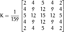
相比直接的使用密度函数来分配权重,Opencv介绍的高斯算子是各像素点乘以一个大于1的比重,最后乘以一个\(1 \frac {159}\),其实就是归一化的密度函数.这有效避免了计算机计算的精度问题



我们在此处直接使用\(3\times3\)的算子

我们将其归一化然后代入上面的代码即可

def GaussianOperator(roi):
    GaussianKernel = np.array([[1,2,1],[2,4,2],[1,2,1]])
    result = np.sum(roi*GaussianKernel/16)
    return result

def GaussianSmooth(image):
    new_image = np.zeros(image.shape)
    image = cv2.copyMakeBorder(image,1,1,1,1,cv2.BORDER_DEFAULT)
    for i in range(1,image.shape[0]-1):
        for j in range(1,image.shape[1]-1):
            new_image[i-1,j-1] =GaussianOperator(image[i-1:i+2,j-1:j+2])
    return new_image.astype(np.uint8)

smooth_saber = GaussianSmooth(gray_saber)
plt.subplot(121)
plt.title("Origin Image")
plt.axis("off")
plt.imshow(gray_saber,cmap="gray")
plt.subplot(122)
plt.title("GaussianSmooth Image")
plt.axis("off")
plt.imshow(smooth_saber,cmap="gray")
plt.show()

计算梯度幅值和方向

我们知道边缘实质是颜色变换的极值,可能出现在各个方向上,因此能否在计算时考虑多个方向的梯度,是算法效果优异的体现之一

在之前的Sobel等算子中我们将水平和垂直方向是分开考虑的.在Canny算子中利用下面公式将多个方向都考虑到

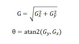
Gx = SobelAlogrithm(smooth_saber,"horizontal")
Gy = SobelAlogrithm(smooth_saber,"vertical")

G = np.sqrt(np.square(Gx.astype(np.float64))+np.square(Gy.astype(np.float64)))
cita = np.arctan2(Gy.astype(np.float64),Gx.astype(np.float64))

cita求出了图像每一个点的梯度,在之后的非极大值抑制中会有作用

plt.imshow(G.astype(np.uint8),cmap="gray")
plt.axis("off")
plt.show()

我们发现对于图像使用sobel算子使得获得的边缘较粗,下一步我们将使图像的线条变细

非最大值抑制

在获得梯度的方向和大小之后，应该对整幅图想做一个扫描，出去那些非边界上的点。对每一个像素进行检查，看这个点的梯度是不是周围具有相同梯度方向的点中最大的。



(图像来源于opencv官方文档)

非极大值的算法实现非常简单

• 比较当前点的梯度强度和正负梯度方向点的梯度强度。
• 如果当前点的梯度强度和同方向的其他点的梯度强度相比较是最大，保留其值。否则抑制，即设为0。比如当前点的方向指向正上方90°方向，那它需要和垂直方向，它的正上方和正下方的像素比较。

def NonmaximumSuppression(image,cita):
    keep = np.zeros(cita.shape)
    cita = np.abs(cv2.copyMakeBorder(cita,1,1,1,1,cv2.BORDER_DEFAULT))
    for i in range(1,cita.shape[0]-1):
        for j in range(1,cita.shape[1]-1):
            if cita[i][j]>cita[i-1][j] and cita[i][j]>cita[i+1][j]:
                keep[i-1][j-1] = 1
            elif cita[i][j]>cita[i][j+1] and cita[i][j]>cita[i][j-1]:
                keep[i-1][j-1] = 1
            elif cita[i][j]>cita[i+1][j+1] and cita[i][j]>cita[i-1][j-1]:
                keep[i-1][j-1] = 1
            elif cita[i][j]>cita[i-1][j+1] and cita[i][j]>cita[i+1][j-1]:
                keep[i-1][j-1] = 1
            else:
                keep[i-1][j-1] = 0
    return keep*image

这里的代码我们先创建了一个keep矩阵,凡是在cita中梯度大于周边的点设为1,否则设为0,然后与原图相乘.(这是我想得比较巧妙的一个方法)

nms_image = NonmaximumSuppression(G,cita)
nms_image = (nms_image*(255/np.max(nms_image))).astype(np.uint8)

plt.imshow(nms_image,cmap="gray")
plt.axis("off")
plt.show()

在上面的极大值抑制中我们使边缘的线变得非常细,但是仍然有相当多的小点,得使用一种算法将他们去除

滞后阈值

滞后阈值的算法如下

Canny 使用了滞后阈值，滞后阈值需要两个阈值(高阈值和低阈值):

• 如果某一像素位置的幅值超过 高 阈值, 该像素被保留为边缘像素。
• 如果某一像素位置的幅值小于 低 阈值, 该像素被排除。
• 如果某一像素位置的幅值在两个阈值之间,该像素仅仅在连接到一个高于 高 阈值的像素时被保留。

在opencv官方文档中推荐我们用2:1或3:1的高低阈值.

我们使用3:1的阈值来进行滞后阈值算法.

滞后阈值的算法可以分成两步首先使用最大阈值,最小阈值排除掉部分点.

MAXThreshold = np.max(nms_image)/4*3
MINThreshold = np.max(nms_image)/4
usemap = np.zeros(nms_image.shape)
high_list = []

for i in range(nms_image.shape[0]):
    for j in range(nms_image.shape[1]):
        if nms_image[i,j]>MAXThreshold:
            high_list.append((i,j))

direct = [(0,1),(1,1),(-1,1),(-1,-1),(1,-1),(1,0),(-1,0),(0,-1)]
def DFS(stepmap,start):
    route = [start]
    while route:
        now = route.pop()
        if usemap[now] == 1:
            break
        usemap[now] = 1
        for dic in direct:
            next_coodinate = (now[0]+dic[0],now[1]+dic[1])
            if not usemap[next_coodinate] and nms_image[next_coodinate]>MINThreshold \
            and next_coodinate[0]<stepmap.shape[0]-1 and next_coodinate[0]>=0 \
            and next_coodinate[1]<stepmap.shape[1]-1 and next_coodinate[1]>=0:
                route.append(next_coodinate)

for i in high_list:
    DFS(nms_image,i)

plt.imshow(nms_image*usemap,cmap="gray")
plt.axis("off")
plt.show()

可以发现这次的效果并不好,这是由于最大最小阈值设定不是很好导致的,我们将上面代码整理,将最大阈值,最小阈值改为可变参数,调参来优化效果.

Canny边缘检测代码

def CannyAlogrithm(image,MINThreshold,MAXThreshold):
    image = GaussianSmooth(image)
    Gx = SobelAlogrithm(image,"horizontal")
    Gy = SobelAlogrithm(image,"vertical")
    G = np.sqrt(np.square(Gx.astype(np.float64))+np.square(Gy.astype(np.float64)))
    G = G*(255/np.max(G)).astype(np.uint8)
    cita = np.arctan2(Gy.astype(np.float64),Gx.astype(np.float64))
    nms_image = NonmaximumSuppression(G,cita)
    nms_image = (nms_image*(255/np.max(nms_image))).astype(np.uint8)
    usemap = np.zeros(nms_image.shape)
    high_list = []
    for i in range(nms_image.shape[0]):
        for j in range(nms_image.shape[1]):
            if nms_image[i,j]>MAXThreshold:
                high_list.append((i,j))

    direct = [(0,1),(1,1),(-1,1),(-1,-1),(1,-1),(1,0),(-1,0),(0,-1)]
    def DFS(stepmap,start):
        route = [start]
        while route:
            now = route.pop()
            if usemap[now] == 1:
                break
            usemap[now] = 1
            for dic in direct:
                next_coodinate = (now[0]+dic[0],now[1]+dic[1])
                if next_coodinate[0]<stepmap.shape[0]-1 and next_coodinate[0]>=0 \
                and next_coodinate[1]<stepmap.shape[1]-1 and next_coodinate[1]>=0 \
                and not usemap[next_coodinate] and nms_image[next_coodinate]>MINThreshold:
                    route.append(next_coodinate)
    for i in high_list:
        DFS(nms_image,i)
    return nms_image*usemap

我们试着调整阈值,来对其他图片进行检测

通过调整阈值可以减少毛点的存在,控制线的清晰

(PS:在使用canny过程中为了减少python运算的时间,我将图片进行了缩放,这也导致了效果不够明显,canny边缘检测在高分辨率情况下效果会更好)

参考资料

Opencv文档

stackoverflow

Numpy设计的是如此出色,以至于在实现算法时我能够忽略如此之多无关的细节