Python GDAL读取栅格数据并基于质量评估波段QA对指定数据加以筛选掩膜
本文介绍基于Python语言中gdal模块,对遥感影像数据进行栅格读取与计算,同时基于QA波段对像元加以筛选、掩膜的操作。
本文所要实现的需求具体为:现有自行计算的全球叶面积指数(LAI).tif格式栅格产品(下称“自有产品”),为了验证其精确度,需要与已有学者提出的成熟产品——GLASS全球LAI.hdf格式栅格产品(下称“GLASS产品”)进行做差对比;其中,自有产品除了LAI波段外,还有一个质量评估波段(QA),即自有产品在后期使用时,还需结合QA波段进行筛选、掩膜等处理。其中,二者均为基于MODIS hv分幅的产品。
本文分为两部分,第一部分为代码的详细分段讲解,第二部分为完整代码。
1 代码分段讲解
1.1 模块与路径准备
首先,需要对用到的模块与存放栅格图像的各类路径加以准备。
import os

import copy

import numpy as np

import pylab as plt

from osgeo import gdal

# rt_file_path="G:/Postgraduate/LAI_Glass_RTlab/Rc_Lai_A2018161_h12v03.tif"

# gl_file_path="G:/Postgraduate/LAI_Glass_RTlab/GLASS01E01.V50.A2018161.h12v03.2020323.hdf"

# out_file_path="G:/Postgraduate/LAI_Glass_RTlab/test.tif"

rt_file_path="I:/LAI_RTLab/A2018161/"

gl_file_path="I:/LAI_Glass/2018161/"

out_file_path="I:/LAI_Dif/"
其中,rt_file_path为自有产品的存放路径,gl_file_path为GLASS产品的存放路径,out_file_path为最终二者栅格做完差值处理后结果的存放路径。
1.2 栅格图像文件名读取与配对
接下来,需要将全部待处理的栅格图像用os.listdir()进行获取,并用for循环进行循环批量处理操作的准备。
rt_file_list=os.listdir(rt_file_path)

for rt_file in rt_file_list:

    file_name_split=rt_file.split("_")

    rt_hv=file_name_split[3][:-4]

    gl_file_list=os.listdir(gl_file_path)

    for gl_file in gl_file_list:

        if rt_hv in gl_file:

            rt_file_tif_path=rt_file_path+rt_file

            gl_file_tif_path=gl_file_path+gl_file
其中,由于本文需求是对两种产品做差,因此首先需要结合二者的hv分幅编号,将同一分幅编号的两景遥感影像放在一起;因此,依据自有产品文件名的特征,选择.split()进行字符串分割,并随后截取获得遥感影像的hv分幅编号。
1.3 输出文件名称准备
前述1.1部分已经配置好了输出文件存放的路径,但是还没有进行输出文件文件名的配置;因此这里我们需要配置好每一个做差后的遥感影像的文件存放路径与名称。其中,我们就直接以遥感影像的hv编号作为输出结果文件名。
            DRT_out_file_path=out_file_path+"DRT/"

            if not os.path.exists(DRT_out_file_path):

                os.makedirs(DRT_out_file_path)

            DRT_out_file_tif_path=os.path.join(DRT_out_file_path,rt_hv+".tif")

            eco_out_file_path=out_file_path+"eco/"

            if not os.path.exists(eco_out_file_path):

                os.makedirs(eco_out_file_path)

            eco_out_file_tif_path=os.path.join(eco_out_file_path,rt_hv+".tif")

            wat_out_file_path=out_file_path+"wat/"

            if not os.path.exists(wat_out_file_path):

                os.makedirs(wat_out_file_path)

            wat_out_file_tif_path=os.path.join(wat_out_file_path,rt_hv+".tif")

            tim_out_file_path=out_file_path+"tim/"

            if not os.path.exists(tim_out_file_path):

                os.makedirs(tim_out_file_path)

            tim_out_file_tif_path=os.path.join(tim_out_file_path,rt_hv+".tif")
这一部分代码分为了四个部分,是因为自有产品的LAI是分别依据四种算法得到的,在做差时需要每一种算法分别和GLASS产品进行相减,因此配置了四个输出路径文件夹。
1.4 栅格文件数据与信息读取
接下来,利用gdal模块对.tif与.hdf等两种栅格图像加以读取。
            rt_raster=gdal.Open(rt_file_path+rt_file)

            rt_band_num=rt_raster.RasterCount

            rt_raster_array=rt_raster.ReadAsArray()

            rt_lai_array=rt_raster_array[0]

            rt_qa_array=rt_raster_array[1]

            rt_lai_band=rt_raster.GetRasterBand(1)

            # rt_lai_nodata=rt_lai_band.GetNoDataValue()

            # rt_lai_nodata=32767

            # rt_lai_mask=np.ma.masked_equal(rt_lai_array,rt_lai_nodata)

            rt_lai_array_mask=np.where(rt_lai_array>30000,np.nan,rt_lai_array)

            rt_lai_array_fin=rt_lai_array_mask*0.001

            gl_raster=gdal.Open(gl_file_path+gl_file)

            gl_band_num=gl_raster.RasterCount

            gl_raster_array=gl_raster.ReadAsArray()

            gl_lai_array=gl_raster_array

            gl_lai_band=gl_raster.GetRasterBand(1)

            gl_lai_array_mask=np.where(gl_lai_array>1000,np.nan,gl_lai_array)

            gl_lai_array_fin=gl_lai_array_mask*0.01

            row=rt_raster.RasterYSize

            col=rt_raster.RasterXSize

            geotransform=rt_raster.GetGeoTransform()

            projection=rt_raster.GetProjection()
首先,以上述代码的第一段为例进行讲解。其中,gdal.Open()读取栅格图像;.RasterCount获取栅格图像波段数量;.ReadAsArray()将栅格图像各波段的信息读取为Array格式,当波段数量大于1时,其共有三维,第一维为波段的个数;rt_raster_array[0]表示取Array中的第一个波段,在本文中也就是自有产品的LAI波段;rt_qa_array=rt_raster_array[1]则表示取出第二个波段,在本文中也就是自有产品的QA波段;.GetRasterBand(1)表示获取栅格图像中的第一个波段(注意,这里序号不是从0开始而是从1开始);np.where(rt_lai_array>30000,np.nan,rt_lai_array)表示利用np.where()函数对Array中第一个波段中像素>30000加以选取,并将其设置为nan,其他值不变。这一步骤是消除图像中填充值、Nodata值的方法。最后一句*0.001是将图层原有的缩放系数复原。
其次,上述代码第三段为获取栅格行、列数与投影变换信息。
1.5 差值计算与QA波段筛选
接下来,首先对自有产品与GLASS产品加以做差操作,随后需要对四种算法分别加以提取。
            lai_dif=rt_lai_array_fin-gl_lai_array_fin

            lai_dif=lai_dif*1000

            rt_qa_array_bin=copy.copy(rt_qa_array)

            rt_qa_array_row,rt_qa_array_col=rt_qa_array.shape

            for i in range(rt_qa_array_row):

                for j in range(rt_qa_array_col):

                    rt_qa_array_bin[i][j]="{:012b}".format(rt_qa_array_bin[i][j])[-4:]

            # DRT_pixel_pos=np.where((rt_qa_array_bin>=100) & (rt_qa_array_bin==11))

            # eco_pixel_pos=np.where((rt_qa_array_bin<100) & (rt_qa_array_bin==111))

            # wat_pixel_pos=np.where((rt_qa_array_bin<1000) & (rt_qa_array_bin==1011))

            # tim_pixel_pos=np.where((rt_qa_array_bin<1100) & (rt_qa_array_bin==1111))

            # colormap=plt.cm.Greens

            # plt.figure(1)

            # # plt.subplot(2,4,1)

            # plt.imshow(rt_lai_array_fin,cmap=colormap,interpolation='none')

            # plt.title("RT_LAI")

            # plt.colorbar()

            # plt.figure(2)

            # # plt.subplot(2,4,2)

            # plt.imshow(gl_lai_array_fin,cmap=colormap,interpolation='none')

            # plt.title("GLASS_LAI")

            # plt.colorbar()

            # plt.figure(3)

            # dif_colormap=plt.cm.get_cmap("Spectral")

            # plt.imshow(lai_dif,cmap=dif_colormap,interpolation='none')

            # plt.title("Difference_LAI (RT-GLASS)")

            # plt.colorbar()

            DRT_lai_dif_array=np.where((rt_qa_array_bin>=100) | (rt_qa_array_bin==11),

                                       np.nan,lai_dif)

            eco_lai_dif_array=np.where((rt_qa_array_bin<100) | (rt_qa_array_bin==111),

                                       np.nan,lai_dif)

            wat_lai_dif_array=np.where((rt_qa_array_bin<1000) | (rt_qa_array_bin==1011),

                                       np.nan,lai_dif)

            tim_lai_dif_array=np.where((rt_qa_array_bin<1100) | (rt_qa_array_bin==1111),

                                       np.nan,lai_dif)

            # plt.figure(4)

            # plt.imshow(DRT_lai_dif_array)

            # plt.colorbar()

            # plt.figure(5)

            # plt.imshow(eco_lai_dif_array)

            # plt.colorbar()

            # plt.figure(6)

            # plt.imshow(wat_lai_dif_array)

            # plt.colorbar()

            # plt.figure(7)

            # plt.imshow(tim_lai_dif_array)

            # plt.colorbar()
其中,上述代码前两句为差值计算与数据化整。将数据转换为整数,可以减少结果数据图层的数据量(因为不需要存储小数了)。
随后,开始依据QA波段进行数据筛选与掩膜。其实各类遥感影像(例如MODIS、Landsat等)的QA波段都是比较近似的:通过一串二进制码来表示遥感影像的质量、信息等,其中不同的比特位往往都代表着一种特性。例如下图所示为Landsat Collection 2 Level-2的QA波段含义。
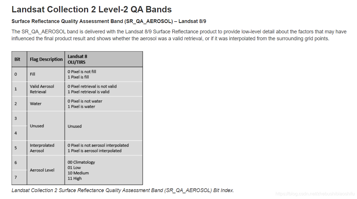
在这里,QA波段原本为十进制(一般遥感影像为了节省空间,QA波段都是写成十进制的形式),因此需要将其转换为二进制;随后通过获取指定需要的二进制数据位数(在本文中也就是能确定自有产品中这一像素来自于哪一种算法的二进制位数),从而判断这一像素所得LAI是通过哪一种算法得到的,从而将每种算法对应的像素分别放在一起处理。DRT_lai_dif_array等四个变量分别表示四种算法中,除了自己这一种算法得到的像素之外的其他所有像素;之所以选择这种方式,是因为后期我们可以将其直接掩膜掉,那么剩下的就是这种算法自身的像素了。
其中,上述代码注释掉的plt相关内容可以实现绘制空间分布图,大家感兴趣可以尝试使用。
1.6 结果栅格文件写入与保存
接下来,将我们完成上述差值计算与依据算法进行筛选后的图像保存。
            driver=gdal.GetDriverByName("Gtiff")

            out_DRT_lai=driver.Create(DRT_out_file_tif_path,row,col,1,gdal.GDT_Float32)

            out_DRT_lai.SetGeoTransform(geotransform)

            out_DRT_lai.SetProjection(projection)

            out_DRT_lai.GetRasterBand(1).WriteArray(DRT_lai_dif_array)

            out_DRT_lai=None

            driver=gdal.GetDriverByName("Gtiff")

            out_eco_lai=driver.Create(eco_out_file_tif_path,row,col,1,gdal.GDT_Float32)

            out_eco_lai.SetGeoTransform(geotransform)

            out_eco_lai.SetProjection(projection)

            out_eco_lai.GetRasterBand(1).WriteArray(eco_lai_dif_array)

            out_eco_lai=None

            driver=gdal.GetDriverByName("Gtiff")

            out_wat_lai=driver.Create(wat_out_file_tif_path,row,col,1,gdal.GDT_Float32)

            out_wat_lai.SetGeoTransform(geotransform)

            out_wat_lai.SetProjection(projection)

            out_wat_lai.GetRasterBand(1).WriteArray(wat_lai_dif_array)

            out_wat_lai=None

            driver=gdal.GetDriverByName("Gtiff")

            out_tim_lai=driver.Create(tim_out_file_tif_path,row,col,1,gdal.GDT_Float32)

            out_tim_lai.SetGeoTransform(geotransform)

            out_tim_lai.SetProjection(projection)

            out_tim_lai.GetRasterBand(1).WriteArray(tim_lai_dif_array)

            out_tim_lai=None

            print(rt_hv)
其中,.GetDriverByName("Gtiff")表示保存为.tif格式的GeoTIFF文件;driver.Create(DRT_out_file_tif_path,row,col,1,gdal.GDT_Float32)表示按照路径、行列数、波段数与数据格式等建立一个新的栅格图层,作为输出图层的框架;其后表示分别将地理投影转换信息与像素具体数值分别赋予这一新建的栅格图层;最后=None表示将其从内存空间中释放,完成写入与保存工作。
2 完整代码
本文所需完整代码如下:
# -*- coding: utf-8 -*-

"""

Created on Thu Jul 15 19:36:15 2021

@author: fkxxgis

"""

import os

import copy

import numpy as np

import pylab as plt

from osgeo import gdal

# rt_file_path="G:/Postgraduate/LAI_Glass_RTlab/Rc_Lai_A2018161_h12v03.tif"

# gl_file_path="G:/Postgraduate/LAI_Glass_RTlab/GLASS01E01.V50.A2018161.h12v03.2020323.hdf"

# out_file_path="G:/Postgraduate/LAI_Glass_RTlab/test.tif"

rt_file_path="I:/LAI_RTLab/A2018161/"

gl_file_path="I:/LAI_Glass/2018161/"

out_file_path="I:/LAI_Dif/"

rt_file_list=os.listdir(rt_file_path)

for rt_file in rt_file_list:

    file_name_split=rt_file.split("_")

    rt_hv=file_name_split[3][:-4]

    gl_file_list=os.listdir(gl_file_path)

    for gl_file in gl_file_list:

        if rt_hv in gl_file:

            rt_file_tif_path=rt_file_path+rt_file

            gl_file_tif_path=gl_file_path+gl_file

            DRT_out_file_path=out_file_path+"DRT/"

            if not os.path.exists(DRT_out_file_path):

                os.makedirs(DRT_out_file_path)

            DRT_out_file_tif_path=os.path.join(DRT_out_file_path,rt_hv+".tif")

            eco_out_file_path=out_file_path+"eco/"

            if not os.path.exists(eco_out_file_path):

                os.makedirs(eco_out_file_path)

            eco_out_file_tif_path=os.path.join(eco_out_file_path,rt_hv+".tif")

            wat_out_file_path=out_file_path+"wat/"

            if not os.path.exists(wat_out_file_path):

                os.makedirs(wat_out_file_path)

            wat_out_file_tif_path=os.path.join(wat_out_file_path,rt_hv+".tif")

            tim_out_file_path=out_file_path+"tim/"

            if not os.path.exists(tim_out_file_path):

                os.makedirs(tim_out_file_path)

            tim_out_file_tif_path=os.path.join(tim_out_file_path,rt_hv+".tif")

            rt_raster=gdal.Open(rt_file_path+rt_file)

            rt_band_num=rt_raster.RasterCount

            rt_raster_array=rt_raster.ReadAsArray()

            rt_lai_array=rt_raster_array[0]

            rt_qa_array=rt_raster_array[1]

            rt_lai_band=rt_raster.GetRasterBand(1)

            # rt_lai_nodata=rt_lai_band.GetNoDataValue()

            # rt_lai_nodata=32767

            # rt_lai_mask=np.ma.masked_equal(rt_lai_array,rt_lai_nodata)

            rt_lai_array_mask=np.where(rt_lai_array>30000,np.nan,rt_lai_array)

            rt_lai_array_fin=rt_lai_array_mask*0.001

            gl_raster=gdal.Open(gl_file_path+gl_file)

            gl_band_num=gl_raster.RasterCount

            gl_raster_array=gl_raster.ReadAsArray()

            gl_lai_array=gl_raster_array

            gl_lai_band=gl_raster.GetRasterBand(1)

            gl_lai_array_mask=np.where(gl_lai_array>1000,np.nan,gl_lai_array)

            gl_lai_array_fin=gl_lai_array_mask*0.01

            row=rt_raster.RasterYSize

            col=rt_raster.RasterXSize

            geotransform=rt_raster.GetGeoTransform()

            projection=rt_raster.GetProjection()

            lai_dif=rt_lai_array_fin-gl_lai_array_fin

            lai_dif=lai_dif*1000

            rt_qa_array_bin=copy.copy(rt_qa_array)

            rt_qa_array_row,rt_qa_array_col=rt_qa_array.shape

            for i in range(rt_qa_array_row):

                for j in range(rt_qa_array_col):

                    rt_qa_array_bin[i][j]="{:012b}".format(rt_qa_array_bin[i][j])[-4:]

            # DRT_pixel_pos=np.where((rt_qa_array_bin>=100) & (rt_qa_array_bin==11))

            # eco_pixel_pos=np.where((rt_qa_array_bin<100) & (rt_qa_array_bin==111))

            # wat_pixel_pos=np.where((rt_qa_array_bin<1000) & (rt_qa_array_bin==1011))

            # tim_pixel_pos=np.where((rt_qa_array_bin<1100) & (rt_qa_array_bin==1111))

            # colormap=plt.cm.Greens

            # plt.figure(1)

            # # plt.subplot(2,4,1)

            # plt.imshow(rt_lai_array_fin,cmap=colormap,interpolation='none')

            # plt.title("RT_LAI")

            # plt.colorbar()

            # plt.figure(2)

            # # plt.subplot(2,4,2)

            # plt.imshow(gl_lai_array_fin,cmap=colormap,interpolation='none')

            # plt.title("GLASS_LAI")

            # plt.colorbar()

            # plt.figure(3)

            # dif_colormap=plt.cm.get_cmap("Spectral")

            # plt.imshow(lai_dif,cmap=dif_colormap,interpolation='none')

            # plt.title("Difference_LAI (RT-GLASS)")

            # plt.colorbar()

            DRT_lai_dif_array=np.where((rt_qa_array_bin>=100) | (rt_qa_array_bin==11),

                                       np.nan,lai_dif)

            eco_lai_dif_array=np.where((rt_qa_array_bin<100) | (rt_qa_array_bin==111),

                                       np.nan,lai_dif)

            wat_lai_dif_array=np.where((rt_qa_array_bin<1000) | (rt_qa_array_bin==1011),

                                       np.nan,lai_dif)

            tim_lai_dif_array=np.where((rt_qa_array_bin<1100) | (rt_qa_array_bin==1111),

                                       np.nan,lai_dif)

            # plt.figure(4)

            # plt.imshow(DRT_lai_dif_array)

            # plt.colorbar()

            # plt.figure(5)

            # plt.imshow(eco_lai_dif_array)

            # plt.colorbar()

            # plt.figure(6)

            # plt.imshow(wat_lai_dif_array)

            # plt.colorbar()

            # plt.figure(7)

            # plt.imshow(tim_lai_dif_array)

            # plt.colorbar()

            driver=gdal.GetDriverByName("Gtiff")

            out_DRT_lai=driver.Create(DRT_out_file_tif_path,row,col,1,gdal.GDT_Float32)

            out_DRT_lai.SetGeoTransform(geotransform)

            out_DRT_lai.SetProjection(projection)

            out_DRT_lai.GetRasterBand(1).WriteArray(DRT_lai_dif_array)

            out_DRT_lai=None

            driver=gdal.GetDriverByName("Gtiff")

            out_eco_lai=driver.Create(eco_out_file_tif_path,row,col,1,gdal.GDT_Float32)

            out_eco_lai.SetGeoTransform(geotransform)

            out_eco_lai.SetProjection(projection)

            out_eco_lai.GetRasterBand(1).WriteArray(eco_lai_dif_array)

            out_eco_lai=None

            driver=gdal.GetDriverByName("Gtiff")

            out_wat_lai=driver.Create(wat_out_file_tif_path,row,col,1,gdal.GDT_Float32)

            out_wat_lai.SetGeoTransform(geotransform)

            out_wat_lai.SetProjection(projection)

            out_wat_lai.GetRasterBand(1).WriteArray(wat_lai_dif_array)

            out_wat_lai=None

            driver=gdal.GetDriverByName("Gtiff")

            out_tim_lai=driver.Create(tim_out_file_tif_path,row,col,1,gdal.GDT_Float32)

            out_tim_lai.SetGeoTransform(geotransform)

            out_tim_lai.SetProjection(projection)

            out_tim_lai.GetRasterBand(1).WriteArray(tim_lai_dif_array)

            out_tim_lai=None

            print(rt_hv)
至此,大功告成。
Python GDAL读取栅格数据并基于质量评估波段QA对指定数据加以筛选掩膜的更多相关文章
- python gdal 读取栅格数据
1.gdal包简介 gdal是空间数据处理的开源包,其支持超过100种栅格数据类型,涵盖所有主流GIS与RS数据格式,包括Arc/Info ASCII Grid(asc),GeoTiff (tiff) ...
- python实现六大分群质量评估指标(兰德系数、互信息、轮廓系数)
python实现六大分群质量评估指标(兰德系数.互信息.轮廓系数) 1 R语言中的分群质量--轮廓系数 因为先前惯用R语言,那么来看看R语言中的分群质量评估,节选自笔记︱多种常见聚类模型以及分群质量评 ...
- Python GDAL矢量转栅格详解
前言:挺久没有更新博客了,前段时间课程实验中需要用代码将矢量数据转成栅格,常见的点栅格化方法通过计算将点坐标(X,Y)转换到格网坐标(I,J),线栅格化方法主要有DDA算法.Bresenham算法等, ...
- GDAL读取的坐标起点在像素左上角还是像素中心?
目录 1. 问题 2. 结论 3. 例外 1. 问题 笔者在处理地理栅格数据的时候,总是会发生偏差半个像素的问题. 比如说通过ArcMap打开一张.tif,查看其地理信息:同时用记事本打开.tfw,比 ...
- OpenCV + python 实现人脸检测(基于照片和视频进行检测)
OpenCV + python 实现人脸检测(基于照片和视频进行检测) Haar-like 通俗的来讲,就是作为人脸特征即可. Haar特征值反映了图像的灰度变化情况.例如:脸部的一些特征能由矩形特征 ...
- TOP100summit:【分享实录-Microsoft】基于Kafka与Spark的实时大数据质量监控平台
本篇文章内容来自2016年TOP100summit Microsoft资深产品经理邢国冬的案例分享.编辑:Cynthia 邢国冬(Tony Xing):Microsoft资深产品经理.负责微软应用与服 ...
- python gdal安装与简单使用
原文链接:python gdal安装与简单使用 gdal安装方式一:在网址 https://www.lfd.uci.edu/~gohlke/pythonlibs/#gdal 下载对应python版本的 ...
- 视频质量评估学习Note
术语"编解码器 Coder/Decoder"是压缩器/解压缩器或编码器/解码器一词的缩写.顾名思义,编码可使视频文件变小以进行存储,然后在需要再次使用时将压缩后的数据转换成可用的图 ...
- 使用C#版本GDAL读取复数图像
GDAL的C#版本虽然在很多算法接口没有导出,但是在读写数据中的接口基本上都是完全导出了.使用ReadRaster和WriteRaster方法来进行读写,同时对这两个方法进行了重载,对于常用的数据类型 ...
- python下读取excel文件
项目中要用到这个,所以记录一下. python下读取excel文件方法多种,用的是普通的xlrd插件,因为它各种版本的excel文件都可读. 首先在https://pypi.python.org/py ...
随机推荐
- 2. 第一个PyQt5 程序 Helloword!
专栏地址 ʅ(‾◡◝)ʃ 第一个 PyQt5 程序 2.1 import sys from PyQt5.QtWidgets import QApplication,QWidget app = QApp ...
- python3爬取CSDN个人所有文章列表页
前言 我之前写了下载单篇文章的接口函数,结合这篇写的,就可以下载所有个人的所有文章了 代码实现 没什么技术含量就是简单的 xpath 处理,不过有意思的是有一位csdn 员工将自己的博客地址写到源码里 ...
- PostgreSQL:查询元数据(表 、字段)信息、库表导入导出命令
一.查询表.模式及字段信息 1.查询指定模式下的所有表 select tablename,* from pg_tables where schemaname = 'ods'; 2.查询指定模式下的表名 ...
- 《MySQL必知必会》之事务、用户权限、数据库维护和性能
第二十六章 管理事务处理 本章介绍什么是事务处理以及如何利用COMMIT和ROLLBACK语句来管理事务处理 事务处理 并非所有数据库引擎都支持事务处理 常用的InnoDB支持 事务处理可以用来维护数 ...
- Effective C++试读笔记
Part1 习惯C++ 1. 视C++为一个语言联邦 C++非常的屌,除了开发效率和编译效率不高,其他的都非常屌 C++ 可以视为一系列的语言联邦构成的紧密结合体,分为以下四个部分 C 2.C wit ...
- texlive安装与vscode环境配置
环境 系统:windows10 texlive下载 下载地址: 官网:http://tug.org/texlive/ 清华镜像源: https://mirrors.tuna.tsinghua.edu. ...
- Python函数用法和底层分析
目录 Python函数用法和底层分析 函数的基本概念 Python 函数的分类 核心要点 形参和实参 文档字符串(函数的注释) 返回值 函数也是对象,内存底层分析 变量的作用域(全局变量和局部变量) ...
- VMware搭建内网渗透环境
网络结构: 攻击机:kali 192.168.1.103 DMZ区域:防火墙 WAN:192.168.1.104 LAN:192.168.10.10 winserver03 LAN:192.168.1 ...
- SSM框架——MyBatis
Mybatis 1.Mybatis的使用 1.1给项目导入相关依赖 我这里有几个下载好的依赖包提供给大家 点我下载--junit4.13.2 点我下载--maven3.8.1 点我下载--mybati ...
- 区块链特辑——solidity语言基础(七)
Solidity语法基础学习 十.实战项目(二): 3.项目实操: ERC20 代币实战 ①转账篇 总发行量函数 totalSupply() return(uint256) ·回传代币的发行总量 ·使 ...