Link Analysis_2_Application

US Cities Distribution Network

1.1 Task Description

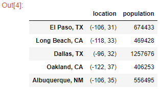
Nodes: Cities with attributes (1) location, (2) population;

Edges: Connections between cities with weight attribute the cost of traveling;

%matplotlib notebook
import networkx as nx
import matplotlib.pyplot as plt
G = nx.read_gpickle('major_us_cities')

G.nodes(data=True)

[('El Paso, TX', {'location': (-106, 31), 'population': 674433}),
 ('Long Beach, CA', {'location': (-118, 33), 'population': 469428}),
 ('Dallas, TX', {'location': (-96, 32), 'population': 1257676}),
 ('Oakland, CA', {'location': (-122, 37), 'population': 406253}),
 ('Albuquerque, NM', {'location': (-106, 35), 'population': 556495}),
 ('Baltimore, MD', {'location': (-76, 39), 'population': 622104}),
 ('Raleigh, NC', {'location': (-78, 35), 'population': 431746}),
 ('Mesa, AZ', {'location': (-111, 33), 'population': 457587}),
 ('Arlington, TX', {'location': (-97, 32), 'population': 379577}),
 ('Sacramento, CA', {'location': (-121, 38), 'population': 479686}),
 ('Wichita, KS', {'location': (-97, 37), 'population': 386552}),
 ('Tucson, AZ', {'location': (-110, 32), 'population': 526116}),
 ('Cleveland, OH', {'location': (-81, 41), 'population': 390113}),
 ('Louisville/Jefferson County, KY',
  {'location': (-85, 38), 'population': 609893}),
 ('San Jose, CA', {'location': (-121, 37), 'population': 998537}),
 ('Oklahoma City, OK', {'location': (-97, 35), 'population': 610613}),
 ('Atlanta, GA', {'location': (-84, 33), 'population': 447841}),
 ('New Orleans, LA', {'location': (-90, 29), 'population': 378715}),
 ('Miami, FL', {'location': (-80, 25), 'population': 417650}),
 ('Fresno, CA', {'location': (-119, 36), 'population': 509924}),
 ('Philadelphia, PA', {'location': (-75, 39), 'population': 1553165}),
 ('Houston, TX', {'location': (-95, 29), 'population': 2195914}),
 ('Boston, MA', {'location': (-71, 42), 'population': 645966}),
 ('Kansas City, MO', {'location': (-94, 39), 'population': 467007}),
 ('San Diego, CA', {'location': (-117, 32), 'population': 1355896}),
 ('Chicago, IL', {'location': (-87, 41), 'population': 2718782}),
 ('Charlotte, NC', {'location': (-80, 35), 'population': 792862}),
 ('Washington D.C.', {'location': (-77, 38), 'population': 646449}),
 ('San Antonio, TX', {'location': (-98, 29), 'population': 1409019}),
 ('Phoenix, AZ', {'location': (-112, 33), 'population': 1513367}),
 ('San Francisco, CA', {'location': (-122, 37), 'population': 837442}),
 ('Memphis, TN', {'location': (-90, 35), 'population': 653450}),
 ('Los Angeles, CA', {'location': (-118, 34), 'population': 3884307}),
 ('New York, NY', {'location': (-74, 40), 'population': 8405837}),
 ('Denver, CO', {'location': (-104, 39), 'population': 649495}),
 ('Omaha, NE', {'location': (-95, 41), 'population': 434353}),
 ('Seattle, WA', {'location': (-122, 47), 'population': 652405}),
 ('Portland, OR', {'location': (-122, 45), 'population': 609456}),
 ('Tulsa, OK', {'location': (-95, 36), 'population': 398121}),
 ('Austin, TX', {'location': (-97, 30), 'population': 885400}),
 ('Minneapolis, MN', {'location': (-93, 44), 'population': 400070}),
 ('Colorado Springs, CO', {'location': (-104, 38), 'population': 439886}),
 ('Fort Worth, TX', {'location': (-97, 32), 'population': 792727}),
 ('Indianapolis, IN', {'location': (-86, 39), 'population': 843393}),
 ('Las Vegas, NV', {'location': (-115, 36), 'population': 603488}),
 ('Detroit, MI', {'location': (-83, 42), 'population': 688701}),
 ('Nashville-Davidson, TN', {'location': (-86, 36), 'population': 634464}),
 ('Milwaukee, WI', {'location': (-87, 43), 'population': 599164}),
 ('Columbus, OH', {'location': (-82, 39), 'population': 822553}),
 ('Virginia Beach, VA', {'location': (-75, 36), 'population': 448479}),
 ('Jacksonville, FL', {'location': (-81, 30), 'population': 842583})]

1.2 Create Layouts for Plotting

Dictionary for node positioning methods:

[x for x in nx.__dir__() if x.endswith('_layout')]

['circular_layout',
 'random_layout',
 'shell_layout',
 'spring_layout',
 'spectral_layout',
 'fruchterman_reingold_layout']

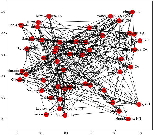
1.2.1 Spring Layout (default) Node Positioning: (1) As few crossing edges as possible; (2) Keep edge length similar.

plt.figure(figsize=(10,9))
nx.draw_networkx(G)

1.2.2 Random Layout

plt.figure(figsize=(10,9))
pos = nx.random_layout(G)
nx.draw_networkx(G, pos)

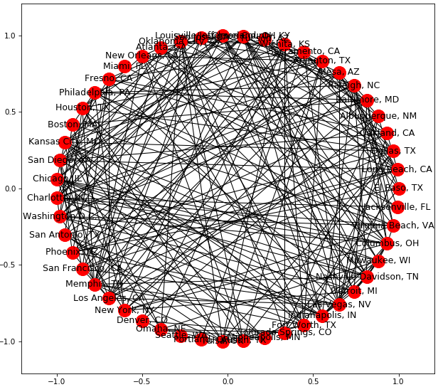
1.2.3 Cicular Layout

plt.figure(figsize=(10,9))
pos = nx.circular_layout(G)
nx.draw_networkx(G, pos)

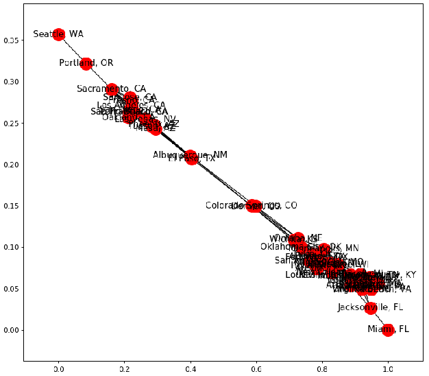
1.2.4 Custom Layout

plt.figure(figsize=(10,7))
pos = nx.get_node_attributes(G, 'location')
nx.draw_networkx(G, pos)

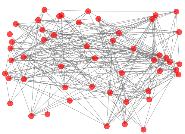
plt.figure(figsize=(10,7))
nx.draw_networkx(G, pos, alpha=0.7, with_labels=False, edge_color='.4')
plt.axis('off')
plt.tight_layout();

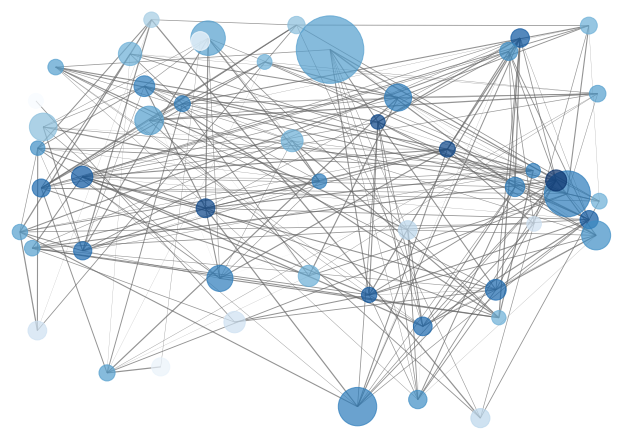
Set size of nodes based on population, multiply pop with small number so plots won't be large.

Get weights of transportation costs and pass it to edges.

plt.figure(figsize=(10,7))
node_color = [G.degree(v) for v in G]
node_size = [0.0005 * nx.get_node_attributes(G, 'population')[v] for v in G]
edge_width = [0.0015*G[u][v]['weight'] for u,v in G.edges()]
nx.draw_networkx(G, pos, node_size=node_size,
                 node_color=node_color, alpha=0.7, with_labels=False,
                 width=edge_width, edge_color='.4', cmap=plt.cm.Blues)
plt.axis('off')
plt.tight_layout();

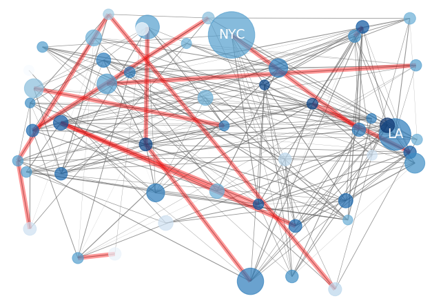
Display the most expensive costs, i.e., separately add specific labels and edges.

plt.figure(figsize=(10,7))
node_color = [G.degree(v) for v in G]
node_size = [0.0005*nx.get_node_attributes(G, 'population')[v] for v in G]
edge_width = [0.0015*G[u][v]['weight'] for u,v in G.edges()]
nx.draw_networkx(G, pos, node_size=node_size,
                 node_color=node_color, alpha=0.7, with_labels=False,
                 width=edge_width, edge_color='.4', cmap=plt.cm.Blues)
greater_than_770 = [x for x in G.edges(data=True) if x[2]['weight']>770]
nx.draw_networkx_edges(G, pos, edgelist=greater_than_770, edge_color='r', alpha=0.4, width=6)
nx.draw_networkx_labels(G, pos, labels={'Los Angeles, CA': 'LA', 'New York, NY': 'NYC'}, font_size=18, font_color='w')
plt.axis('off')
plt.tight_layout();

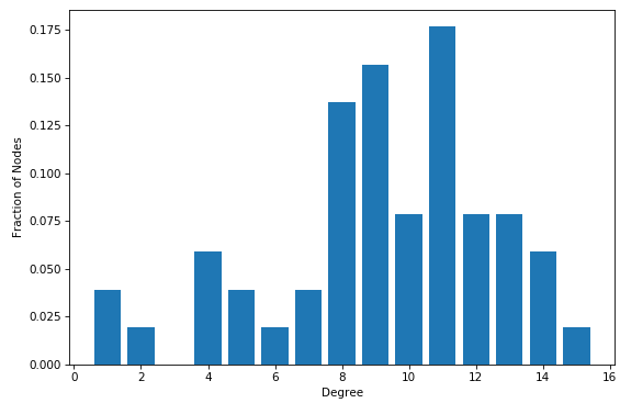
1.3 Degree Distribution

Probability distributions over entire network

# function degree() returns a dictionary with keys being nodes and
# values being degrees of nodes
degrees = G.degree()
degree_values = sorted(set(degrees.values()))
histogram = [list(degrees.values()).count(i)/float(nx.number_of_nodes(G)) for i in degree_values]
import matplotlib.pyplot as plt
plt.bar(degree_values, histogram)
plt.xlabel('Degree')
plt.ylabel('Fraction of Nodes')
plt.show()

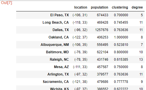
1.4 Extracting Attributes

1.4.1 Node-based Method

Transform into DataFrame columns, initialize the dataframe, using the nodes as the index:

df = pd.DataFrame(index = G.nodes())

df['location'] = pd.Series(nx.get_node_attributes(G, 'location'))
df['population'] = pd.Series(nx.get_node_attributes(G, 'population'))
df.head()

Add features:

df['clustering'] = pd.Series(nx.clustering(G))
df['degree'] = pd.Series(G.degree())
df

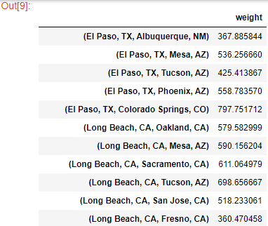
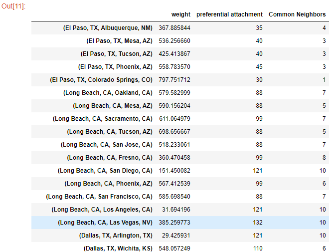
1.4.2 Edge-based Features

Initialize the DataFrame, using the edges as the index:

G.edges(data=True)
df = pd.DataFrame(index=G.edges())
df['weight'] = pd.Series(nx.get_edge_attributes(G, 'weight'))
df

df['preferential attachment'] = [i[2] for i in nx.preferential_attachment(G, df.index)]
df['Common Neighbors'] = df.index.map(lambda city: len(list(nx.common_neighbors(G, city[0], city[1]))))
df