Morphological Image Processing

概
- reflection and translation
Erosion and Dilation
Opening and Closing
The Hit-or-Miss Transform
一些基本的操作
Morphological Reconstruction

Gonzalez R. C. and Woods R. E. Digital Image Processing (Forth Edition)

符号	即	操作	说明
$\ominus$	erosion	$\{z:(B)_z \subset A\}$	Erodes the boundary of A
$\oplus$	dilation	$\{z:(\hat{B})_z \bigcap A \not= \empty\}$	Dilates the boundary of A
$\circ$	opening	$(A \ominus B) \oplus B$	Smoothes contours, breaks narrow isthmuses, and eliminates small islands and sharp peaks.
$\bullet$	closing	$(A\oplus B) \ominus B$	Smoothes contours, fuses narrow breaks and long thin gulfs, and eliminates small holes.
$\circledast$	hit-or-miss	$\{z:(B)_z \subset I\}$	Finds I. B contains instances both of foreground B in image and background elements.
$\beta(A)$	boundary extraction	$A - (A \ominus B)$	Set of points on the boundary of set A
-	hole filling	$(X_{k-1} \oplus B) \bigcap I^c$	Fills holes in A
-	connected components	$(X_{k-1} \oplus B) \bigcap I$	Finds connected components in $I$.
$C(A)$	convex hull	$(X_{k-1}^i \circledast B^i) \bigcup X_{k-1}^i$	Finds the convex hull
$\otimes$	thining	$A - (A \circledast B)$	Thins set A
$\odot$	thickening	$A\bigcup (A \circledast B)$	Thickens set A
$S(A)$	skeleton	$(A \ominus kB) - (A \ominus kB) \circ B $	Finds the skeleton of set A
-	pruning	...	$X_4$ is the result of pruning set A.
$D_G^{(1)}(F)$	geodesic dilation	$(F \oplus B) \bigcap G$	-
$E_G^{(1)}(F)$	geodesic erosion	$(F \ominus B) \bigcup G$	-
$R_G^D(F)$	morphological reconstruction by dilation	$R_G^D (F) = D^{(k)}_G (F)$	-
$R_G^E(F)$	morphological reconstruction by erosion	$R_G^E (F) = E^{(k)}_G (F)$	-
$O_R^{(n)}(F)$	opening by reconstruction	$R_{F}^D (F \ominus nB)$	-
$C_R^{(n)}(F)$	closing by reconstruction	$ R_{F}^E (F \oplus nB)$	-
-	hole filling	$H = [R_{I^c}D(F)]^c $	Auto
-	border clearing	$I - R_I^D(F)$	-

概

直接把整个章节都拿来是决定这个形态学的东西实在是有趣, 加之前后联系过于紧密, 感觉如果过于割裂会导致以后回忆不起来, 所以直接对整个章节做个笔记得了.

我觉得首先需要牢记的是, 本章节是在集合的基础上讨论的, 对于一个二元图中的物体, 我们可以通过如下集合表示:

\[\{(x_1, y_1), \cdots, (x_N, y_N)\},
\]

$(x, y)$表示值为$1$的坐标(这里假设foreground pixel的值为1, 当然也可以假设其为0).

注: 个人觉得, 这里讨论的时候并非像之前的图片一样以左上角原点, 而是以目标中心为原点然后发散开去(只是单纯便于理解和书写, 实际处理是不受影响的). 也就意味着, $x, y$是可以为负的, 显然这种表示的好处是不需要确定整个图片的大小范围.

本章节会频繁涉及到objects和structuring elements (SE)的概念, 说实话其具体的定义不是很清楚, 我还是从任务的角度来给它们做个解释.

因为本章节讨论的transform, 通常都是通过SE经过一些集合操作使得objects发生某种改变, 所以objects就是对象. SE

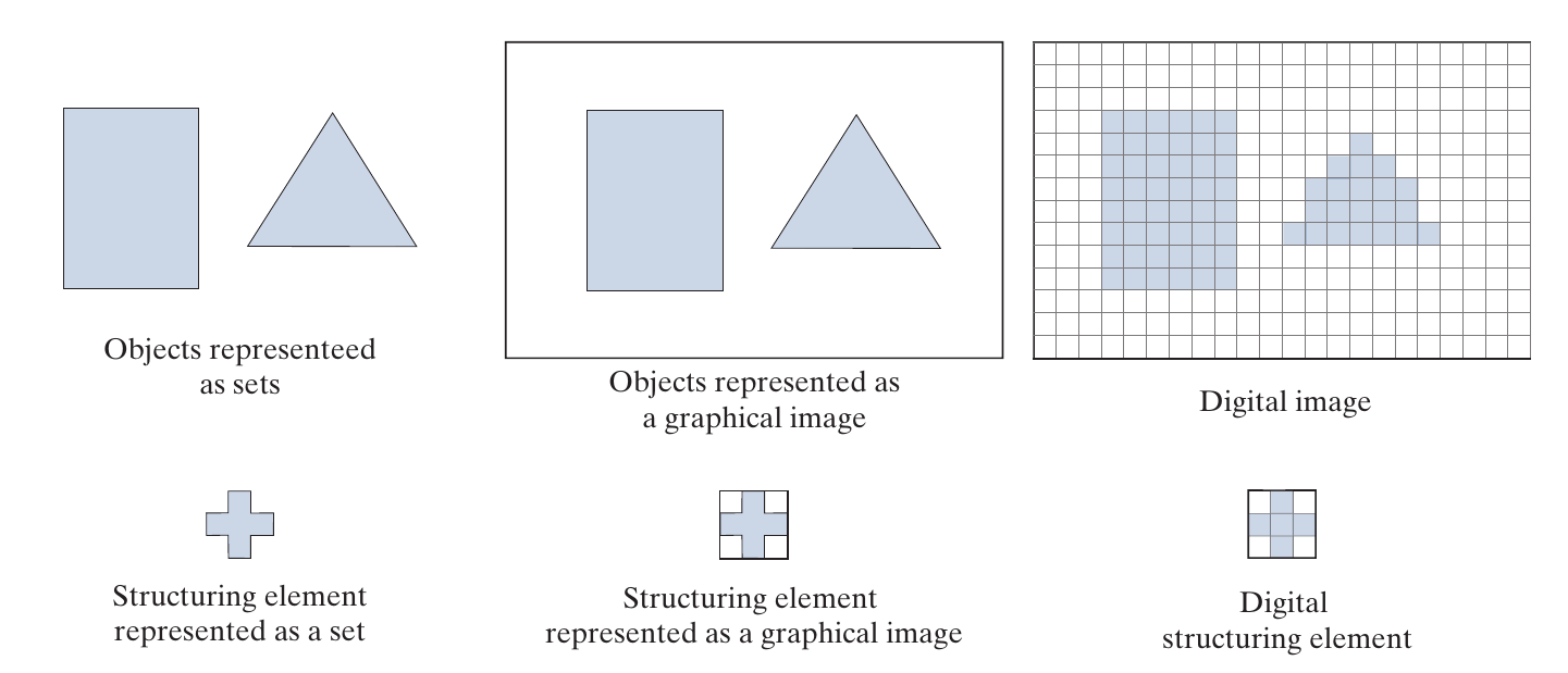
如上图所示, 虽然objects是一个仅仅记录0值的集合, 我们通常将其置于一个矩形区域中, 便于图片的处理, SE也是类似的. 特别的是, SE整体除了0, 1外还可能有$\times$的属性, 其表示0或1, 即该位置的点不我们所关心的点, 其可以任意匹配.

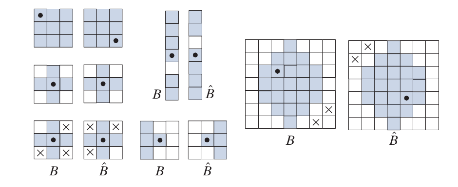
reflection and translation

反射, 即

\[\hat{B} = \{w| w=-b, \text{for } b \in B\},
\]

需要注意的是该反射是以$B$的中心为原点的.

平移, 即

\[(B)_z = \{c| c= b+z, \text{for } b \in B\}.
\]

Erosion and Dilation

Erosion

Erosion操作能够令图片中的元素'缩小', 所以其在处理噪声的时候其实不错. 其定义为:

\[\begin{array}{ll}
A \ominus B &= \{z| (B)_z \subset A\} \\
&= \{w \in Z^2 | w + b \in A \text{ for every } b \in B\} \\
&= \mathop{\bigcap} \limits_{b \in B} (A)_{-b}.
\end{array}
\]

proof:

设上面三个定义分别为$C_1, C_2, C_3$.

$C_1 \subset C_2$:

$\forall z \in C_1$,

\[\{b_1+z, b_2 + z, \cdots\} \subset A,
\]

故

\[z + b \in A, \text{ for every } b \in B \Rightarrow C_1 \subset C_2.
\]

$C_2 = C_3$:

\[C_2 = \{w \in Z^2 | w + b \in A \text{ for every } b \in B\}
=\bigcap_{b \in B} \{a-b \in Z^2 | \in A\}
=\bigcap_{b \in B} (A)_{-b}.
\]

$C_3 \subset C_1$:

$\forall w \in C_2$:

\[(B)_w \subset A \Rightarrow C_3 \subset C_1.
\]

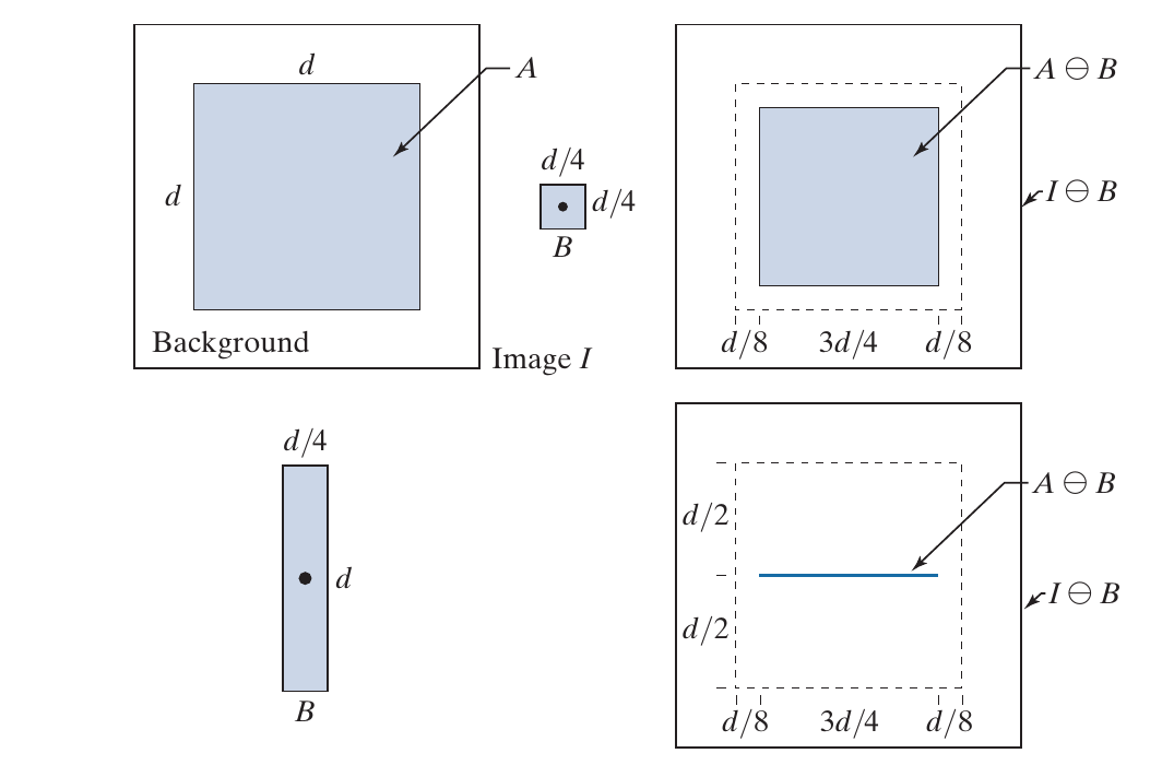
示例

如下图所示, 第一行第一幅图是object, 通过第二幅SE erosion后object缩小了, 而通过第二行的SE更是直接成了一条线.

skimage.morphology.erosion

[erosion](Module: morphology — skimage v0.19.0.dev0 docs (scikit-image.org))

import numpy as np

import matplotlib.pyplot as plt

from skimage.morphology import erosion, disk

def plot_comparison(original, filtered, filter_name):

    fig, (ax1, ax2) = plt.subplots(ncols=2, figsize=(8, 4), sharex=True,

                                   sharey=True)

    ax1.imshow(original, cmap=plt.cm.gray)

    ax1.set_title('original')

    ax1.axis('off')

    ax2.imshow(filtered, cmap=plt.cm.gray)

    ax2.set_title(filter_name)

    ax2.axis('off')

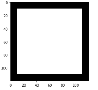
img = np.ones((100, 100))

arow = np.zeros((10, 100))

img = np.vstack((arow, img, arow))

acol = np.zeros((120, 10))

img = np.hstack((acol, img, acol)).astype(np.uint8)

fig, ax = plt.subplots()

ax.imshow(img, cmap=plt.cm.gray)

footprint = disk(6) # {0, 1}, 半径为6的圆, 中心元素为1其余为0

eroded = erosion(img, footprint)

plot_comparison(img, eroded, 'erosion')

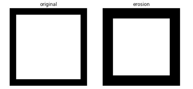
dilation

dilation的效果是令图中的元素进行扩张, 一些扫描的文本图像可能字符剑有断痕, 通过此可以修复.

其集合定义为:

\[\begin{array}{ll}
A \oplus B
&= \{z| (\hat{B})_z \bigcap A \not= \empty\} \\
&= \{w \in Z^2| w = a+ b, \text{ for some } a \in A \text{ and } b \in B\}\\
&= \mathop{\bigcup}_{b \in B} (A)_b \\
&= \mathop{\bigcup}_{a \in A} (B)_a.
\end{array}
\]

proof:

记上面四种定义各自为$C_1, C_2, C_3, C_4$:

$C_1 = C_2$:

$\forall z \in C_1$:

\[\exist a \in A, b \in B, \quad \mathrm{s.t.} \: -b + z = a \rightarrow z = a + b \rightarrow z \in C_2,
\]

故

\[C_1 \subset C_2.
\]

$\forall w \in C_2$:

\[\exist a \in A, b \in B, \quad \mathrm{s.t.} \: w = a+b \rightarrow -b + w = a \rightarrow (\hat{B})_w \bigcap A \not= \empty,
\]

故

\[C_2 \subset C_1.
\]

$C_2 = C_3 = C_4$:

显然.

最后两个定义是很直观的, $C_3$相当于对于每一个点$b\in B$为中心画一个$A$, $C_4$则是以每一个$a \in A$为中心画一个$B$.

示例

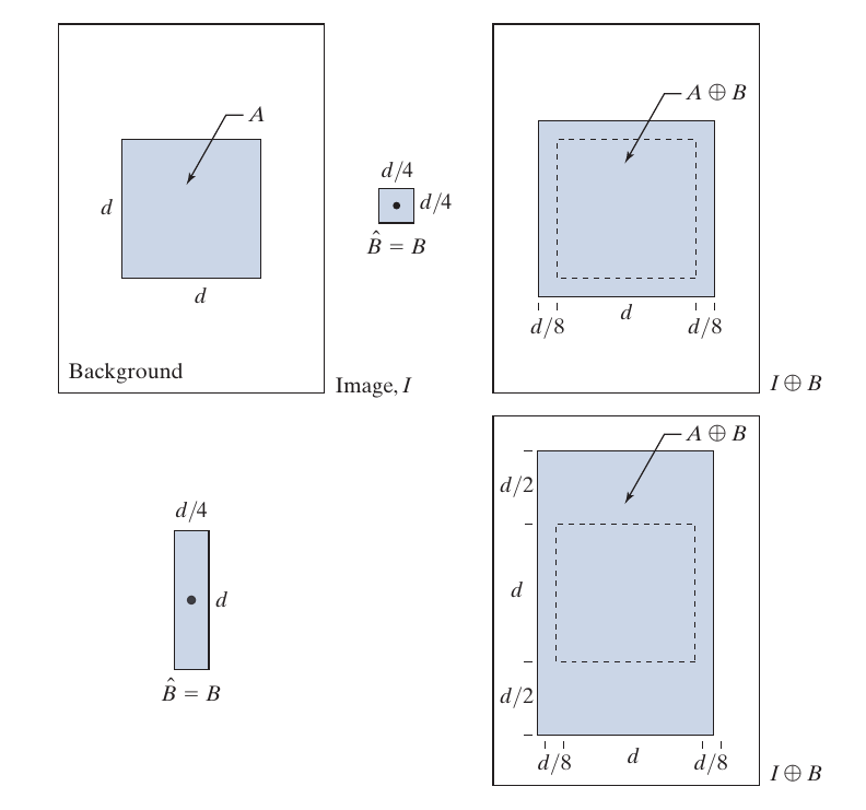
skimage.morphology.dilation

dilation

from skimage.morphology import dilation

footprint = disk(6) # {0, 1}, 半径为6的圆, 中心元素为1其余为0

dilated = dilation(eroded, footprint)

plot_comparison(eroded, dilated, 'dilation')

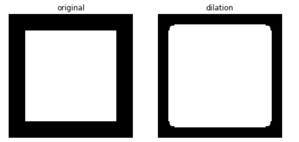
注: 圆角实际上是下一节的东西.

对偶性

\[\begin{array}{ll}
(A\ominus B)^c
&= \{z| (B)_z \subset A\}^c \\
&= \{z| (B)_z \bigcap A^c \not = \empty\} \\
&= A^c \oplus \hat{B}.
\end{array}
\]

\[\begin{array}{ll}
(A\oplus B)^c
&= \{z| (\hat{B})_z \bigcap A \not= \empty \}^c \\
&= \{z| (\hat{B})_z \subset A^c\} \\
&= A^c \ominus \hat{B}.
\end{array}
\]

Opening and Closing

二者都有一种将目标变圆滑的效果.

Opening

定义:

\[A \circ B = (A \ominus B) \oplus B = \mathop{\bigcup} \limits_{z} \{(B)_z | (B)_z \subset A\}.
\]

proof:

\[\begin{array}{ll}
(A \ominus B) \oplus B
&= \bigcup_{z \in A \ominus B} (B)_z \\
&= \bigcup_{z} \{(B)_z| (B)_z \subset A\}.
\end{array}
\]

示例

skimage.morphology.opening

opening

from skimage.morphology import opening

footprint = disk(6)

opened = opening(img, footprint)

plot_comparison(img, opened, 'opening')

Closing

定义:

\[A \bullet B = (A \oplus B) \ominus B = [\bigcup \{(\hat{B})_z| (\hat{B})_z \bigcap A = \empty\}]^c.
\]

注: 书中为:

\[A \bullet B = (A \oplus B) \ominus B = [\bigcup \{(B)_z| (B)_z \bigcap A = \empty\}]^c,
\]

但感觉不一样啊.

proof:

\[\begin{array}{ll}
[(A \oplus B) \ominus B]^c
&= (A \oplus B)^c \oplus \hat{B} \\
&= (A^c \ominus \hat{B}) \oplus \hat{B} \\
&= \bigcup_z \{(\hat{B})_z | (\hat{B})_z \subset A^c\} \\
&= \bigcup_z \{(\hat{B})_z | (\hat{B})_z \bigcap A = \empty\} \\
\end{array}
\]

示例

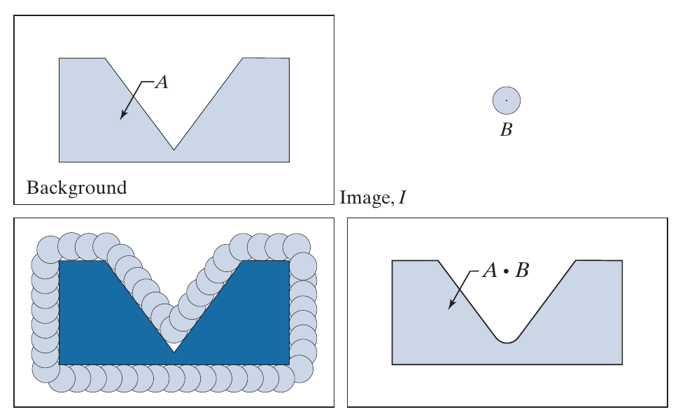
skimage.morphology.closing

closing

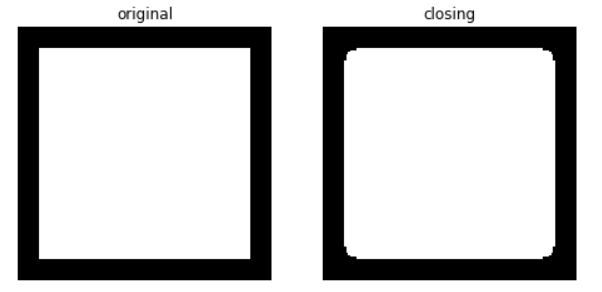
from skimage.morphology import closing

footprint = disk(6)

closed = opening(img, footprint)

plot_comparison(img, closed, 'closing')

对偶性

\[(A \circ B)^c = (A^c \bullet \hat{B}) \\
(A \bullet B)^c = (A^c \circ \hat{B})
\]

且

\[(A \circ B) \circ B = A \circ B \\
(A \bullet B) \bullet B = A \bullet B.
\]

The Hit-or-Miss Transform

主要用于shape detection.

定义:

\[I \circledast B_{1,2} = (A \ominus B_1) \bigcap (A^c \ominus B_2),
\]

此为$B_1, B_2$不包含$0$元素的情形, 倘若允许$B$包含0元素, 那么

\[I \circledast B = I \ominus B,
\]

只是我们$B$通常需要一些特殊的性质来使其具有detection的作用.

具体怎么shape detection 还是请回看原文吧.

一些基本的操作

Boundary Extraction

定义:

\[\beta(A) = A - (A \ominus B)
\]

直观的感觉就是把object的中间部分挖掉.

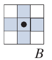
Hole Filling

假设在我们想填的hole中已知一个点, 以这个点为基础出发(记为$X_0$):

\[X_k = (X_{k-1} \oplus B) \bigcap I^c, k=1,2,3,\cdots,
\]

停止准则为

\[X_k = X_{k+1}.
\]

不过需要注意的是, $B$应该选择下面类型的(如果是全满的话可能跳出hole了).

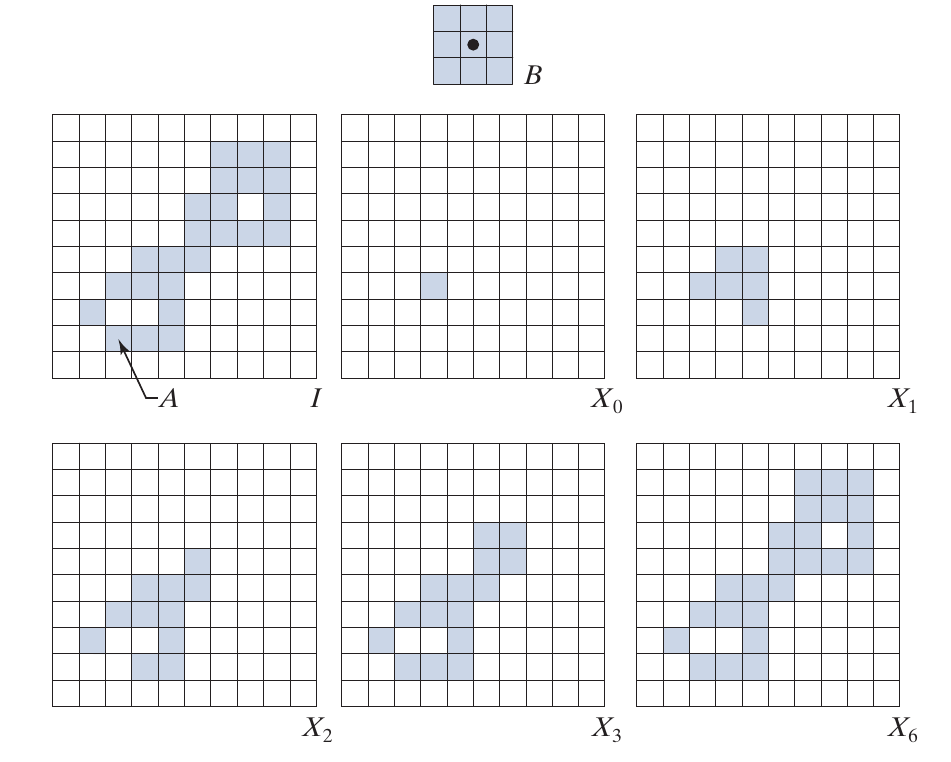
Extraction of Connected Components

抓取连通区域, 假设已知在我们想抓取的连通区域的一点, 从这个点出发(记为$X_0$):

\[X_k = (X_{k-1} \oplus B) \bigcap I, k=1,2,\cdots,
\]

直到

\[X_{k+1} = X_k.
\]

Convex Hull

将一个object填补成凸的, 这个说实话没怎么看明白.

\[X_k^i = (X_{k-1}^i \circledast B^i) \bigcup X_{k-1}^i, i=1,2,3,4, k=1,2,\cdots \\
X_0^i = I.
\]

当

\[X_{k+1}^i = X_{k}^i
\]

时停止, 记其为$D^i$, 最后的convex hull 为

\[C(A) = \mathop{\bigcup}_{i=1}^4 D^i.
\]

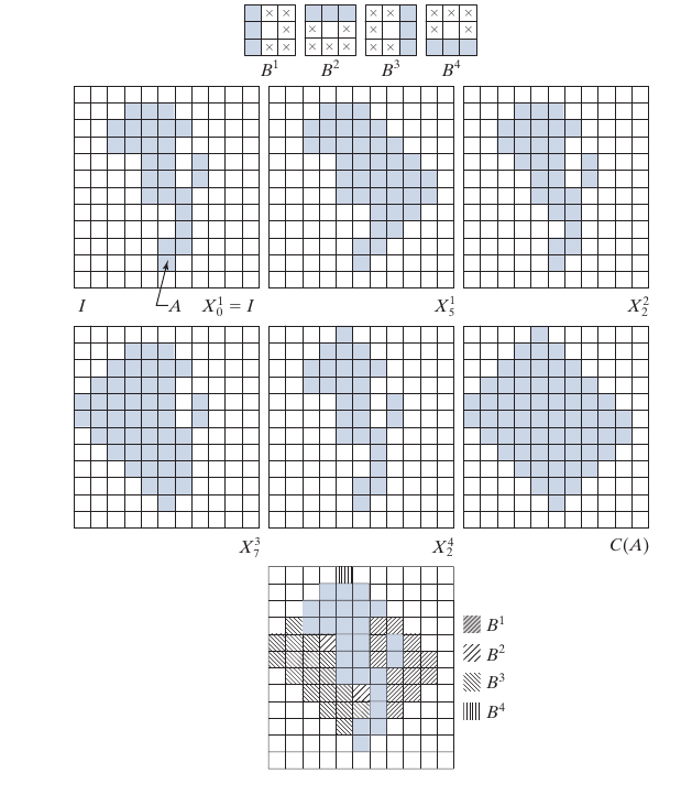
总感觉这个不是最小的凸包啊.

skimage.morphology.convex_hull_image

convex_hull

Thinning

定义:

\[A \otimes B = A - (A \circledast B) = A \bigcap (A \circledast B)^c
\]

skimage.morphology.thin

thin

Thickening

相反的操作:

\[A \odot B = A \bigcup (A \circledast B).
\]

Skeletons

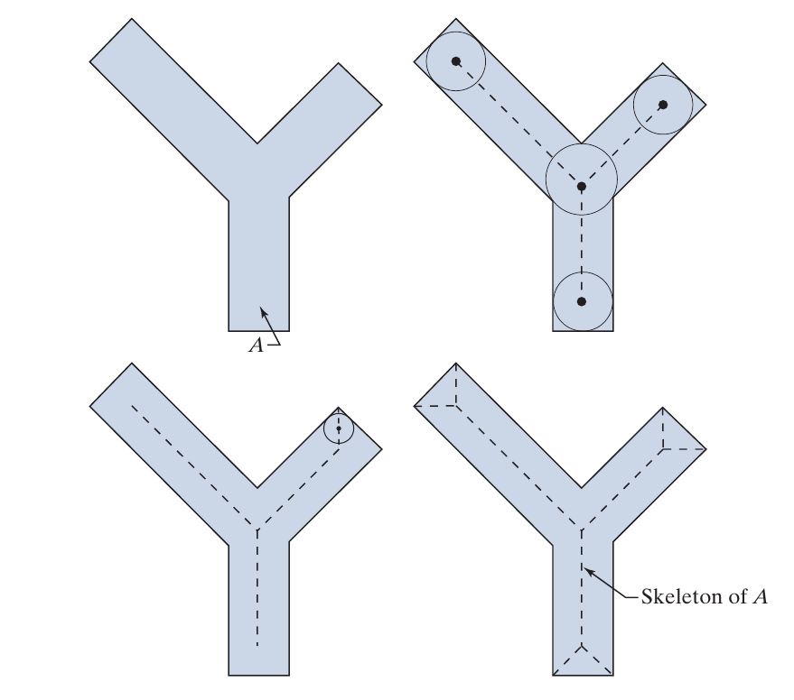
其严格的定义有些复杂, 感觉有点拓扑结构?

\[S(A) = \mathop{\bigcup} \limits_{k=0}^K S_k(A), \\
S_k(A) = (A \ominus kB) - (A \ominus kB) \circ B \\
(A \ominus kB) = ((\ldots ((A\ominus B) \ominus B)\ominus \ldots) \ominus B)\\
K = \max \{k| (A \ominus kB) \not = \empty \}.
\]

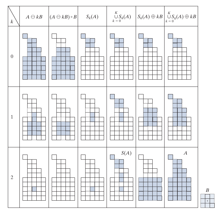
skimage.morphology.skeletonize

skeleton

Pruning

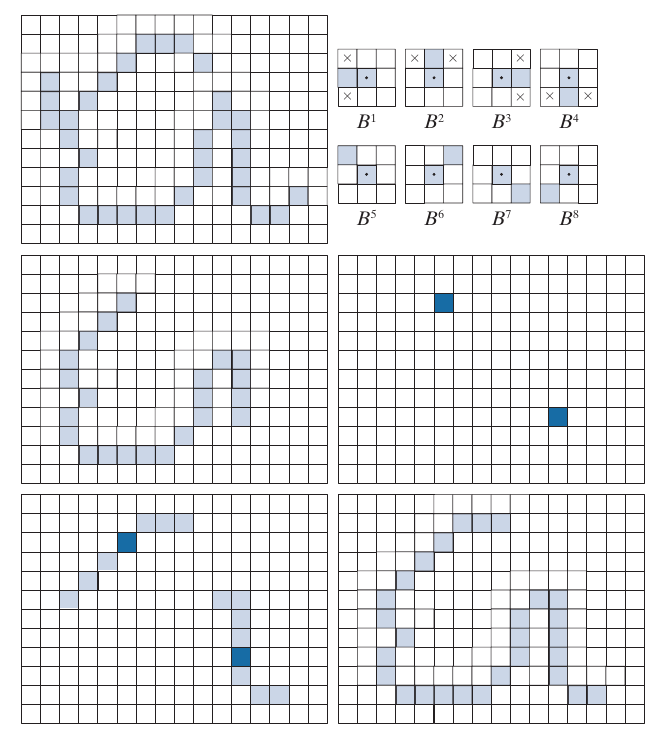
pruning 方法用于去掉别的方法留下的一些spurs:

\[X_1 = A \otimes \{B\} \\
X_2 = \mathop{\bigcup} \limits_{k=1}^8 (X_1 \circledast B^k) \\
X_3 = (X_2 \oplus H) \bigcap A \\
X_4 = X_1 \bigcup X_3.
\]

$B^k$为下图的一系列(而$\{B\}$为其中一部分不一定全部用到):

Morphological Reconstruction

Morphological Reconstruction除了之前用到的$F, B$外, 还要额外用到一个图片(称为mask)作为一个reconstruction的limit.

Geodesic Dilation and Erosion

假设$F \subset G$, geodesic dilation:

\[D_G^{(1)} (F) = (F \oplus B) \bigcap G \\
D_G^{(n)} (F) = D_G^{(1)} (D_G^{(n-1)} (F)), \quad D_G^{(0)} (F) = F.
\]

geodesic erosion:

\[E_G^{(1)}(F) = (F \ominus B) \bigcup G \\
E_G^{(n)}(F) = E_G^{(1)}(E_G^{(n-1)}(F)), \quad E_G^{(0)}(F) = F.
\]

直观上很好解释, 即geodesic dilation在扩张的时候不能超过$G$, 而geodesic erosion在收缩的时候不会少于$G$.

Morphological Reconstruction by Dilation and by Erosion

定义很简单, 即重复上述操作直到收敛:

\[R_G^D (F) = D^{(k)}_G (F), \quad \text{if } D^{(k)}_G (F) = D^{(k-1)}_G (F), \\
R_G^E (F) = E^{(k)}_G (F), \quad \text{if } E^{(k)}_G (F) = E^{(k-1)}_G (F).
\]

Opening|Closing by Reconstruction

\[O_R^{(n)}(F) = R_{F}^D (F \ominus nB),
\]

直观解释就是, 先erosion $n$次, 再在此基础上不断扩张(受限于$F$).

Closing by Reconstruction 就是:

\[C_R^{(n)}(F) = R_{F}^E (F \oplus nB).
\]

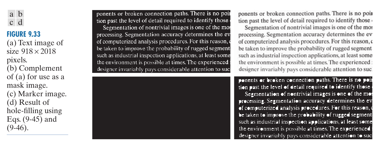
Automatic Algorithm for Filling Holes

之前介绍的hole filling需要一个点为基础, 这个算法是全自动的.

\[F(x, y) =
\left \{
\begin{array}{ll}
1 - I(x, y) & \text{if } (x, y) \text{ is on the border of } I \\
0 & \text{otherwise}.
\end{array}
\right .
\]

\[H = [R_{I^c}^D(F)]^c \\
H \bigcap I^c
\]

感觉还是挺好理解的, 就是从边边, 由于中间部分的hole一定会被包围起来, 所以$H^c$一定不包含中间部分的hole.

Border Clearing

\[F(x, y) =
\left \{
\begin{array}{ll}
I(x, y) & \text{if } (x, y) \text{ is on the border of } I \\
0 & \text{otherwise}.
\end{array}
\right .
\]

\[X = I - R_{I}^D(F).
\]

能够把边缘的一些部分给去了.