Machine Learning week_2 Multivariate Prameters Regression

目录

• 1 Multivariate Prameters Regression
  • 1.1 Reading Multiple Features
  • 1.2 Gradient Descent For Multiple Variables
  • 1.3 Gradient Descent in Practice I - Feature Scaling
  • 1.4 Gradient Descent in Practice II - Learning Rate
  • 1.5 Features and Polynomial Regression
• 2 Computing Parameters Analytically
  • 2.1 Normal Equation
  • 2.2 Normal Equation Noninvertibility
• 3Programming Assignment: Linear Regression

1 Multivariate Prameters Regression

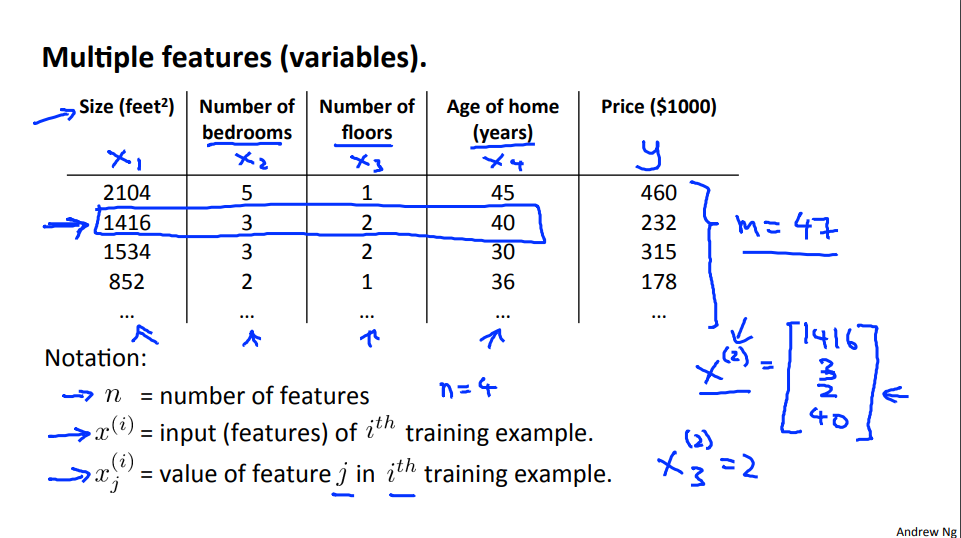
1.1 Reading Multiple Features

Linear regression with multiple variables is also known as "multivariate linear regression".

We now introduce notation for equations where we can have any number of input variables.

\[\begin{align*}x_j^{(i)} &= \text{value of feature } j \text{ in the }i^{th}\text{ training example} \newline x^{(i)}& = \text{the input (features) of the }i^{th}\text{ training example} \newline m &= \text{the number of training examples} \newline n &= \text{the number of features} \end{align*}
\]

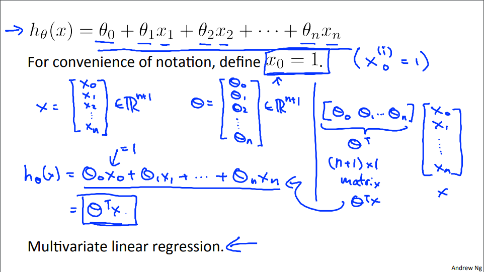
The multivariable form of the hypothesis function accommodating these multiple features is as follows:

\[h_{\theta}(x) = \theta_0 + \theta_1x_1 + \theta_2x_2 + \theta_3x_3 + \; \cdots \;+ \theta_nx_n
\]

In order to develop intuition about this function, we can think about \(\theta_0\) as the basic price of a house, \(\theta_1\) as the price per square meter, \(\theta_2\) as the price per floor, etc. \(x_1\) will be the number of square meters in the house, \(x_2\) the number of floors, etc.

\[h_{\theta}(x) = \theta_0x_0 + \theta_1x_1 + \theta_2x_2 + \theta_3x_3 + \; \cdots \;+ \theta_nx_n
\]

\[\begin{align*}h_\theta(x) =\begin{bmatrix}\theta_0 \hspace{2em} \theta_1 \hspace{2em} ... \hspace{2em} \theta_n\end{bmatrix}\begin{bmatrix}x_0 \newline x_1 \newline \vdots \newline x_n\end{bmatrix}= \theta^T x\end{align*}
\]

I think there's an equation here that \(\theta^Tx = x^T\theta\)? Maybe, but I didn't prove it.

This is a vectorization of our hypothesis function for one training example; see the lessons on vectorization to learn more.

Remark: Note that for convenience reasons in this course we assume \(x_{0}^{(i)} =1 \text{ for } (i\in { 1,\dots, m } )\). This allows us to do matrix operations with theta and x. Hence making the two vectors '\(\theta\)' and \(x^{(i)}\) match each other element-wise (that is, have the same number of elements: n+1).

unfamiliar words

1. multivariate [mʌltɪ'veərɪɪt] adj. 多元的；多变量；
   
   Multivariate Linear regression 多元线性回归

2. multiple [ˈmʌltɪpl] adj. 数量多的；多种多样的
   
   exp： ADJ many in number; involving many different people or things

   • multiple copies of documents
     
     各种文件的大量的副本

   • a multiple entry visa
     
     多次入境签证

   • That works with multiple features.(Form Transcript)

1.2 Gradient Descent For Multiple Variables

\(
Hypothesis: h_{\theta}(x) = \theta_0x_0 + \theta_1x_1 + \theta_2x_2 + \theta_3x_3 + \; \cdots \;+ \theta_nx_n \\
Parameters: \theta_0,\theta_1,\theta_2, \; \cdots \; ,\theta_n \;\Rightarrow \; \theta \in \mathbb{R}^{n+1}\\
Cost\;function: J(\theta_0,\theta_1,\theta_2, \; \cdots \; ,\theta_n)=J(\theta)=\frac{1}{2m} \sum\limits_{i=1}^{m}(h_{\theta}(x^{(i)}) - y^{(i)})^2
\)

Gradient Descent For Multiple Variables

\[\begin{align*} & \text{repeat until convergence:} \; \lbrace \newline \; & \theta_0 := \theta_0 - \alpha \frac{1}{m} \sum\limits_{i=1}^{m} (h_\theta(x^{(i)}) - y^{(i)}) \cdot x_0^{(i)}\newline \; & \theta_1 := \theta_1 - \alpha \frac{1}{m} \sum\limits_{i=1}^{m} (h_\theta(x^{(i)}) - y^{(i)}) \cdot x_1^{(i)} \newline \; & \theta_2 := \theta_2 - \alpha \frac{1}{m} \sum\limits_{i=1}^{m} (h_\theta(x^{(i)}) - y^{(i)}) \cdot x_2^{(i)} \newline & \cdots \newline \rbrace \end{align*}
\\
Simutaneously \; update \; every \;\theta_j \;for j=(0,1,2, \cdots ,n)\]

In other words:

\[\begin{align*}& \text{repeat until convergence:} \; \lbrace \newline \; & \theta_j := \theta_j - \alpha \frac{1}{m} \sum\limits_{i=1}^{m} (h_\theta(x^{(i)}) - y^{(i)}) \cdot x_j^{(i)} \; & \text{for j := 0...n}\newline \rbrace\end{align*}
\]

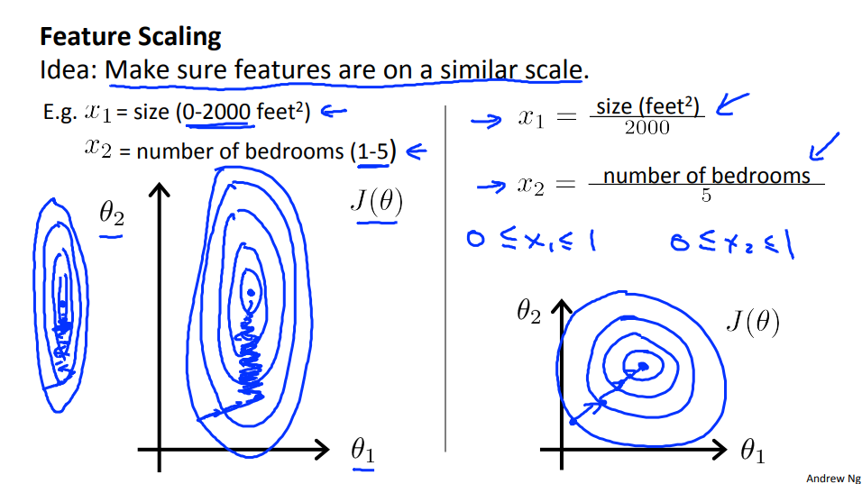
1.3 Gradient Descent in Practice I - Feature Scaling

我还是不太懂为什么，特征缩放会让梯度下降收敛的更快。对于一个线性的h(θ), J(θ)总是一个 convex shape。且拿一个已经拟合好的J(θ)。缩放特征后，数据变成了同一个规模，与此同时，J(θ)中的θ会相应的变大为每个数据的(max-min)倍。这样J(θ)会有非常大的平面，同时，因为梯度下降算法减去的偏导数中，有特征的存在，而这时特征已经非常小了，所以它的迭代速度并不会太快。如果不做特征缩放的话，条件与上面看的一致，这回可能θ小一点，这样J(θ)会有非常小的平面，因为梯度下降算法减去的偏导数中，有特征的存在，若这时特征很大，那么迭代速度也会快速很多。讲义上说 这是因为θ在小范围内迅速下降，在大范围内缓慢下降。因此，当变量非常不均匀时，θ将低效地振荡到最佳值。 这个我得再想想，老师上课也讲的这个例子！

同时课后复习的题目中的答案是 It speed up gradient descent by making it require fewer iterations to get a good solution.

Here's the idea. If you have a problem where you have multiple features, if you make sure that the features are on a similar scale, by which I mean make sure that the different features take on similar ranges of values, then gradient descents can converge more quickly.

We can speed up gradient descent by having each of our input values in roughly the same range. This is because θ will descend quickly on small ranges and slowly on large ranges, and so will oscillate inefficiently down to the optimum when the variables are very uneven.

The way to prevent this is to modify the ranges of our input variables so that they are all roughly the same. Ideally:

\(−1 ≤ x_{(i)} ≤ 1\)

or

\(−0.5 ≤ x_{(i)} ≤ 0.5\)

These aren't exact requirements!!! we are only trying to speed things up. The goal is to get all input variables into roughly one of these ranges, give or take a few.

Two techniques to help with this are feature scaling and mean normalization.

Feature scaling involves dividing the input values by the range (i.e. the maximum value minus the minimum value) of the input variable, resulting in a new range of just 1.

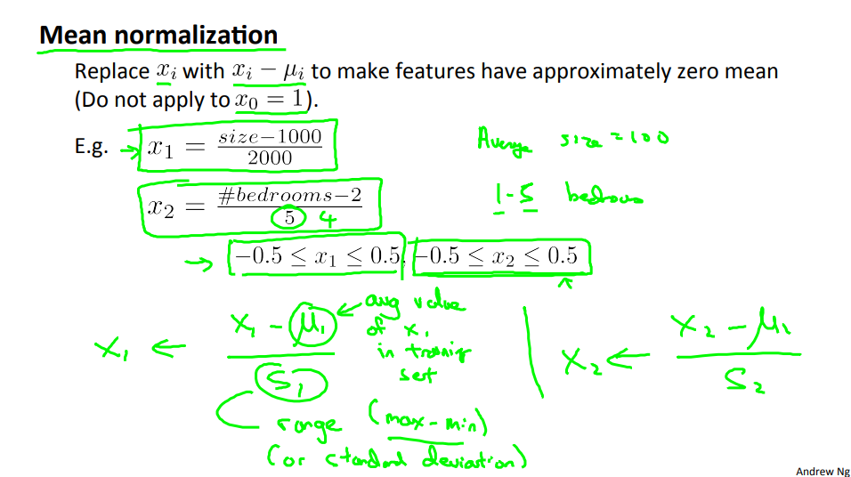
Mean normalization involves subtracting the average value for an input variable from the values for that input variable resulting in a new average value for the input variable of just zero. To implement both of these techniques, adjust your input values as shown in this formula:

\(x_i := \dfrac{x_i - \mu_i}{s_i}\)

Where \(μ_i\) is the average of all the values for feature (i) and \(s_i\) is the range of values (max - min), or \(s_i\) is the standard deviation.(Octave: std())

[Don't apply to \(x_0=1\), if you apply it to \(x_0\), then every \(x_0\) be euqal to 0. So, that would erase the \(\theta_0\) in the \(h_{\theta}\) ]

Note that dividing by the range, or dividing by the standard deviation, give different results. The quizzes in this course use range - the programming exercises use standard deviation.

For example, if \(x_i\) represents housing prices with a range of 100 to 2000 and a mean value of 1000, then, \(x_i := \dfrac{price-1000}{1900}\)

1.4 Gradient Descent in Practice II - Learning Rate

• How to make sure gradient is working correctly?

• How to choose rate α?

So what this plot is showing is, is it's showing the value of your cost function after each iteration of gradient decent. And if gradient is working properly then J(θ) should decrease after every iteration.

If the learning rate is too large, Gradient descent may overshoot the minimum.

And so in order to check your gradient descent's converge I actually tend to look at plots like these, like this figure on the left, rather than rely on an automatic convergence test. Looking at this sort of figure can also tell you, or give you an advance warning, if maybe gradient descent is not working correctly.

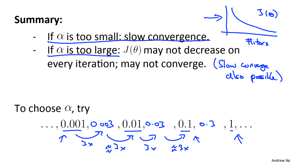
So these are factor of ten differences. And for these different values of alpha are just plot J(θ) as a function of number of iterations, and then pick the value of alpha that seems to be causing J(θ) to decrease rapidly. In fact, what I do actually isn't these steps of ten. So this is a scale factor of ten of each step up. What I actually do is try this range of values. (0.001, 0.003, 0.01, 0.03, 1)

So what I'll do is try a range of values until I've found one value that's too small and made sure that I've found one value that's too large. And then I'll sort of try to pick the largest possible value, or just something slightly smaller than the largest reasonable value that I found. And when I do that usually it just gives me a good learning rate for my problem. And if you do this too, maybe you'll be able to choose a good learning rate for your implementation of gradient descent.

Debugging gradient descent. Make a plot with number of iterations on the x-axis. Now plot the cost function, J(θ) over the number of iterations of gradient descent. If J(θ) ever increases, then you probably need to decrease α.

Automatic convergence test. Declare convergence if J(θ) decreases by less than E in one iteration, where E is some small value such as \(10^{−3}\). However in practice it's difficult to choose this threshold value.

It has been proven that if learning rate α is sufficiently small, then J(θ) will decrease on every iteration.

To summarize:

• If α is too small: slow convergence.

• If α is too large: may not decrease on every iteration and thus may not converge.

1.5 Features and Polynomial Regression

Sometimes very powerful ones by choosing appropriate features.

Sometimes by defining new features you might actually get a better model.

We can improve our features and the form of our hypothesis function in a couple different ways.

We can combine multiple features into one. For example, we can combine \(x_1\) and \(x_2\) into a new feature \(x_3\) by taking \(x_1⋅x_2\)

Polynomial Regression

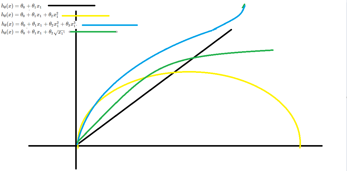
Our hypothesis function need not be linear (a straight line) if that does not fit the data well.

We can change the behavior or curve of our hypothesis function by making it a quadratic, cubic or square root function (or any other form).

For example, if our hypothesis function is s \(h_\theta(x) = \theta_0 + \theta_1 x_1\) then we can create additional features based on \(x_1\) , to get the quadratic function \(h_\theta(x) = \theta_0 + \theta_1 x_1 + \theta_2 x_1^2\) or the cubic function \(h_\theta(x) = \theta_0 + \theta_1 x_1 + \theta_2 x_1^2 + \theta_3 x_1^3\).

In the cubic version, we have created new features x_2 and x_3 where \(x_2 = x_1^2\) and \(x_3 = x_1^3\).

To make it a square root function, we could do: \(h_\theta(x) = \theta_0 + \theta_1 x_1 + \theta_2 \sqrt{x_1}\)

One important thing to keep in mind is, if you choose your features this way then feature scaling becomes very important.

it's important to apply feature scaling if you're using gradient descent to get them into comparable ranges of values.

eg. if \(x_1\) has range 1 - 1000 then range of \(x_1^2\) becomes 1 - 1000000 and that of \(x_1^3\) becomes 1 - 1000000000

2 Computing Parameters Analytically

2.1 Normal Equation

Note: [8:00 to 8:44 - The design matrix X (in the bottom right side of the slide) given in the example should have elements x with subscript 1 and superscripts varying from 1 to m because for all m training sets there are only 2 features \(x_0\) and \(x_1\) 12:56 - The X matrix is m by (n+1) and NOT n by n. ]

Concretely, so far the algorithm that we've been using for linear regression is gradient descent where in order to minimize the cost function J of Theta, we would take this iterative algorithm that takes many steps, multiple iterations of gradient descent to converge to the global minimum. In contrast, the normal equation would give us a method to solve for theta analytically, so that rather than needing to run this iterative algorithm, we can instead just solve for the optimal value for theta all at one go.

Gradient descent gives one way of minimizing J. Let’s discuss a second way of doing so, this time performing the minimization explicitly and without resorting to an iterative algorithm. In the "Normal Equation" method, we will minimize J by explicitly taking its derivatives with respect to the θj ’s, and setting them to zero. This allows us to find the optimum theta without iteration. The normal equation formula is given below:

\[\theta = (X^T X)^{-1}X^Ty
\]

The X matrix is m by (n+1).

There is no need to do feature scaling with the normal equation.

The following is a comparison of gradient descent and the normal equation:

Gradient Descent	Normal Equation
Need to choose alpha	No need to choose alpha
Needs many iterations	No need to iterate
\(O(kn^2)\)	O (n^3), need to calculate inverse of \(X^TX\)
Works well when n is large	Slow if n is very large

With the normal equation, computing the inversion has complexity \(\mathcal{O}(n^3)\), So if we have a very large number of features, the normal equation will be slow. In practice, when n exceeds 10,000 it might be a good time to go from a normal solution to an iterative process.

2.2 Normal Equation Noninvertibility

When implementing the normal equation in octave we want to use the 'pinv' function rather than 'inv.' The 'pinv' function will give you a value \(\theta\) even if \(X^TX\) is not invertible.

if \(X^TX\) is noninvertible, the common causes might be having :

• Redundant features, where two features are very closely related (i.e. they are linearly dependent)

• Too many features (e.g. m ≤ n). In this case, delete some features or use "regularization" (to be explained in a later lesson).

Solutions to the above problems include deleting a feature that is linearly dependent with another or deleting one or more features when there are too many features.

3Programming Assignment: Linear Regression

ex1_Octave.zip