AI - TensorFlow - 示例03：基本回归

基本回归

回归（Regression）：https://www.tensorflow.org/tutorials/keras/basic_regression

主要步骤：
数据部分

1. 获取数据（Get the data）
2. 清洗数据（Clean the data）
3. 划分训练集和测试集（Split the data into train and test）
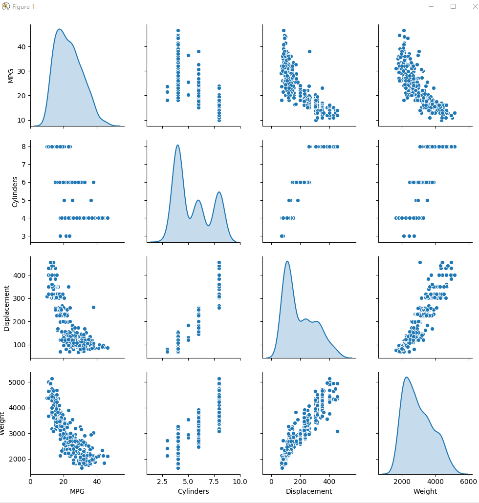
4. 检查数据（Inspect the data）
5. 分离标签（Split features from labels）
6. 规范化数据（Normalize the data）

模型部分

1. 构建模型（Build the model）
2. 检查模型（Inspect the model）
3. 训练模型（Train the model）
4. 做出预测（Make predictions）

Auto MPG Data Set （汽车MPG数据集）

• mpg（miles per gallon, 每加仑行驶的英里数）
• https://archive.ics.uci.edu/ml/datasets/Auto+MPG
• https://archive.ics.uci.edu/ml/machine-learning-databases/auto-mpg/

Attribute Information:

• 1. mpg: continuous
• 2. cylinders: multi-valued discrete
• 3. displacement: continuous
• 4. horsepower: continuous
• 5. weight: continuous
• 6. acceleration: continuous
• 7. model year: multi-valued discrete
• 8. origin: multi-valued discrete
• 9. car name: string (unique for each instance)

一些知识点

验证集

• - 通常指定训练集的一定比例数据作为验证集。
• - 验证集将不参与训练，并在每个epoch结束后测试的模型的指标，如损失函数、精确度等。
• - 如果数据本身是有序的，需要先手工打乱再指定，否则可能会出现验证集样本不均匀。

回调函数(Callbacks)

回调函数是一个函数的合集，在训练的阶段中，用来查看训练模型的内在状态和统计。
在训练时，相应的回调函数的方法就会被在各自的阶段被调用。
一般是在model.fit函数中调用callbacks（参数为callbacks，必须输入list类型的数据）。
简而言之，Callbacks用于指定在每个epoch开始和结束的时候进行哪种特定操作。

• https://keras.io/zh/callbacks/
• https://www.tensorflow.org/api_docs/python/tf/keras/callbacks/

EarlyStopping

EarlyStopping是Callbacks的一种，可用来加快学习的速度，提高调参效率。
使用一个EarlyStopping回调来测试每一个迭代的训练条件，如果某个迭代过后没有显示改进，自动停止训练。

• https://keras.io/zh/callbacks/#earlystopping
• https://www.tensorflow.org/api_docs/python/tf/keras/callbacks/EarlyStopping

结论（conclusion）

• - 均方误差(MSE)是一种常见的损失函数，可用于回归问题。
• - 用于回归和分类问题的损失函数不同，评价指标也不同，常见的回归指标是平均绝对误差(MAE)。
• - 当输入的数据特性包含不同范围的数值，每个特性都应该独立为相同的范围。
• - 如果没有太多的训练数据时，有一个技巧就是采用包含少量隐藏层的小型网络，更适合来避免过拟合。
• - EarlyStopping是一个防止过度拟合的实用技巧。

示例

脚本内容

GitHub：https://github.com/anliven/Hello-AI/blob/master/Google-Learn-and-use-ML/3_basic_regression.py

 # coding=utf-8
 import tensorflow as tf
 from tensorflow import keras
 from tensorflow.python.keras import layers
 import matplotlib.pyplot as plt
 import pandas as pd
 import seaborn as sns
 import pathlib
 import os

 os.environ['TF_CPP_MIN_LOG_LEVEL'] = ''
 print("# TensorFlow version: {}  - tf.keras version: {}".format(tf.VERSION, tf.keras.__version__))  # 查看版本

 # ### 数据部分
 # 获取数据（Get the data）
 ds_path = str(pathlib.Path.cwd()) + "\\datasets\\auto-mpg\\"
 ds_file = keras.utils.get_file(fname=ds_path + "auto-mpg.data", origin="file:///" + ds_path)  # 获得文件路径
 column_names = ['MPG', 'Cylinders', 'Displacement', 'Horsepower', 'Weight', 'Acceleration', 'Model Year', 'Origin']
 raw_dataset = pd.read_csv(filepath_or_buffer=ds_file,  # 数据的路径
                           names=column_names,  # 用于结果的列名列表
                           na_values="?",  # 用于替换NA/NaN的值
                           comment='\t',  # 标识着多余的行不被解析（如果该字符出现在行首，这一行将被全部忽略）
                           sep=" ",  # 分隔符
                           skipinitialspace=True  # 忽略分隔符后的空白（默认为False，即不忽略）
                           )  # 通过pandas导入数据
 data_set = raw_dataset.copy()
 print("# Data set tail:\n{}".format(data_set.tail()))  # 显示尾部数据

 # 清洗数据（Clean the data）
 print("# Summary of NaN:\n{}".format(data_set.isna().sum()))  # 统计NaN值个数（NaN代表缺失值，可用isna()和notna()来检测）
 data_set = data_set.dropna()  # 方法dropna()对缺失的数据进行过滤
 origin = data_set.pop('Origin')  # Origin"列是分类不是数值，转换为独热编码（one-hot encoding）
 data_set['USA'] = (origin == 1) * 1.0
 data_set['Europe'] = (origin == 2) * 1.0
 data_set['Japan'] = (origin == 3) * 1.0
 data_set.tail()
 print("# Data set tail:\n{}".format(data_set.tail()))  # 显示尾部数据

 # 划分训练集和测试集（Split the data into train and test）
 train_dataset = data_set.sample(frac=0.8, random_state=0)
 test_dataset = data_set.drop(train_dataset.index)  # 测试作为模型的最终评估

 # 检查数据（Inspect the data）
 sns.pairplot(train_dataset[["MPG", "Cylinders", "Displacement", "Weight"]], diag_kind="kde")
 plt.figure(num=1)
 plt.savefig("./outputs/sample-3-figure-1.png", dpi=200, format='png')
 plt.show()
 plt.close()
 train_stats = train_dataset.describe()  # 总体统计数据
 train_stats.pop("MPG")
 train_stats = train_stats.transpose()  # 通过transpose()获得矩阵的转置
 print("# Train statistics:\n{}".format(train_stats))

 # 分离标签（Split features from labels）
 train_labels = train_dataset.pop('MPG')  # 将要预测的值
 test_labels = test_dataset.pop('MPG')

 # 规范化数据（Normalize the data）
 def norm(x):
     return (x - train_stats['mean']) / train_stats['std']

 normed_train_data = norm(train_dataset)
 normed_test_data = norm(test_dataset)

 # ### 模型部分
 # 构建模型（Build the model）
 def build_model():  # 模型被包装在此函数中
     model = keras.Sequential([  # 使用Sequential模型
         layers.Dense(64, activation=tf.nn.relu, input_shape=[len(train_dataset.keys())]),  # 包含64个单元的全连接隐藏层
         layers.Dense(64, activation=tf.nn.relu),  # 包含64个单元的全连接隐藏层
         layers.Dense(1)]  # 一个输出层，返回单个连续的值
     )
     optimizer = tf.keras.optimizers.RMSprop(0.001)
     model.compile(loss='mean_squared_error',  # 损失函数
                   optimizer=optimizer,  # 优化器
                   metrics=['mean_absolute_error', 'mean_squared_error']  # 在训练和测试期间的模型评估标准
                   )
     return model

 # 检查模型（Inspect the model）
 mod = build_model()  # 创建模型
 mod.summary()  # 打印出关于模型的简单描述
 example_batch = normed_train_data[:10]  # 从训练集中截取10个作为示例批次
 example_result = mod.predict(example_batch)  # 使用predict()方法进行预测
 print("# Example result:\n{}".format(example_result))

 # 训练模型（Train the model）
 class PrintDot(keras.callbacks.Callback):
     def on_epoch_end(self, epoch, logs):
         if epoch % 100 == 0:
             print('')
         print('.', end='')  # 每完成一次训练打印一个“.”符号

 EPOCHS = 1000  # 训练次数

 history = mod.fit(normed_train_data,
                   train_labels,
                   epochs=EPOCHS,  # 训练周期（训练模型迭代轮次）
                   validation_split=0.2,  # 用来指定训练集的一定比例数据作为验证集（0~1之间的浮点数）
                   verbose=0,  # 日志显示模式：0为安静模式, 1为进度条（默认）, 2为每轮一行
                   callbacks=[PrintDot()]  # 回调函数（在训练过程中的适当时机被调用）
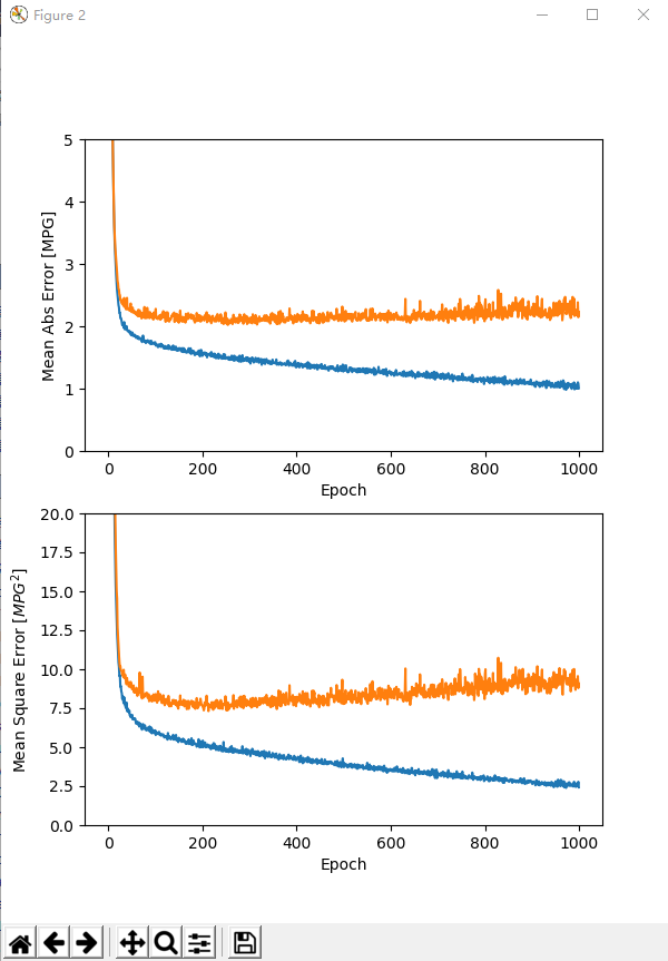
                   )  # 返回一个history对象，包含一个字典，其中包括训练期间发生的情况（training and validation accuracy）

 def plot_history(h, n=1):
     """可视化模型训练过程"""
     hist = pd.DataFrame(h.history)
     hist['epoch'] = h.epoch
     print("\n# History tail:\n{}".format(hist.tail()))

     plt.figure(num=n, figsize=(6, 8))

     plt.subplot(2, 1, 1)
     plt.xlabel('Epoch')
     plt.ylabel('Mean Abs Error [MPG]')
     plt.plot(hist['epoch'], hist['mean_absolute_error'], label='Train Error')
     plt.plot(hist['epoch'], hist['val_mean_absolute_error'], label='Val Error')
     plt.ylim([0, 5])

     plt.subplot(2, 1, 2)
     plt.xlabel('Epoch')
     plt.ylabel('Mean Square Error [$MPG^2$]')
     plt.plot(hist['epoch'], hist['mean_squared_error'], label='Train Error')
     plt.plot(hist['epoch'], hist['val_mean_squared_error'], label='Val Error')
     plt.ylim([0, 20])

     filename = "./outputs/sample-3-figure-" + str(n) + ".png"
     plt.savefig(filename, dpi=200, format='png')
     plt.show()
     plt.close()

 plot_history(history, 2)  # 可视化

 # 调试
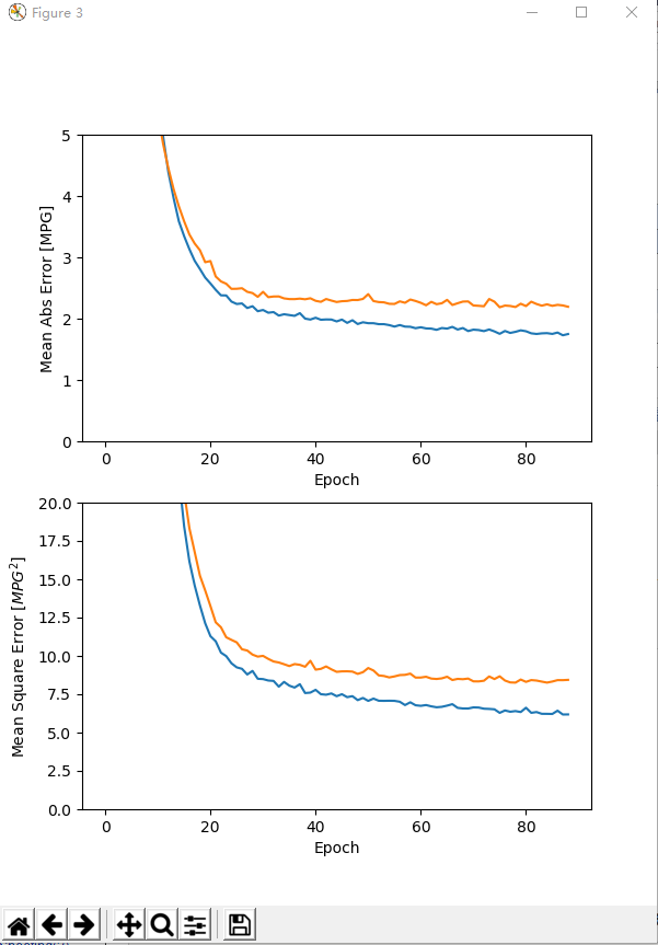
 model2 = build_model()
 early_stop = keras.callbacks.EarlyStopping(monitor='val_loss',
                                            patience=10)  # 指定提前停止训练的callbacks
 history2 = model2.fit(normed_train_data,
                       train_labels,
                       epochs=EPOCHS,
                       validation_split=0.2,
                       verbose=0,
                       callbacks=[early_stop, PrintDot()])  # 当没有改进时自动停止训练（通过EarlyStopping）
 plot_history(history2, 3)
 loss, mae, mse = model2.evaluate(normed_test_data, test_labels, verbose=0)
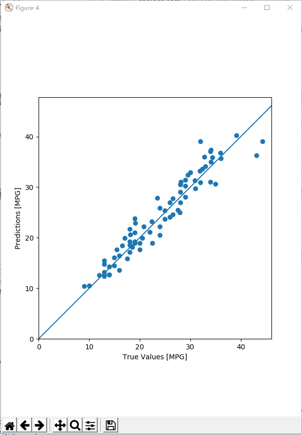
 print("# Testing set Mean Abs Error: {:5.2f} MPG".format(mae))  # 测试集上的MAE值

 # 做出预测（Make predictions）
 test_predictions = model2.predict(normed_test_data).flatten()  # 使用测试集中数据进行预测
 plt.figure(num=4, figsize=(6, 8))
 plt.scatter(test_labels, test_predictions)
 plt.xlabel('True Values [MPG]')
 plt.ylabel('Predictions [MPG]')
 plt.axis('equal')
 plt.axis('square')
 plt.xlim([0, plt.xlim()[1]])
 plt.ylim([0, plt.ylim()[1]])
 plt.plot([-100, 100], [-100, 100])
 plt.savefig("./outputs/sample-3-figure-4.png", dpi=200, format='png')
 plt.show()
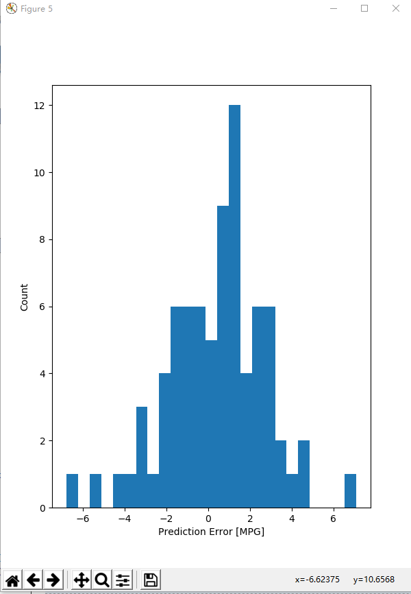
 plt.close()

 error = test_predictions - test_labels
 plt.figure(num=5, figsize=(6, 8))
 plt.hist(error, bins=25)  # 通过直方图来展示错误的分布情况
 plt.xlabel("Prediction Error [MPG]")
 plt.ylabel("Count")
 plt.savefig("./outputs/sample-3-figure-5.png", dpi=200, format='png')
 plt.show()
 plt.close()

运行结果

C:\Users\anliven\AppData\Local\conda\conda\envs\mlcc\python.exe D:/Anliven/Anliven-Code/PycharmProjects/Google-Learn-and-use-ML/3_basic_regression.py
# TensorFlow version: 1.12.0  - tf.keras version: 2.1.6-tf
# Data set tail:
      MPG  Cylinders  Displacement   ...    Acceleration  Model Year  Origin
393  27.0          4         140.0   ...            15.6          82       1
394  44.0          4          97.0   ...            24.6          82       2
395  32.0          4         135.0   ...            11.6          82       1
396  28.0          4         120.0   ...            18.6          82       1
397  31.0          4         119.0   ...            19.4          82       1

[5 rows x 8 columns]
# Summary of NaN:
MPG             0
Cylinders       0
Displacement    0
Horsepower      6
Weight          0
Acceleration    0
Model Year      0
Origin          0
dtype: int64
# Data set tail:
      MPG  Cylinders  Displacement  ...    USA  Europe  Japan
393  27.0          4         140.0  ...    1.0     0.0    0.0
394  44.0          4          97.0  ...    0.0     1.0    0.0
395  32.0          4         135.0  ...    1.0     0.0    0.0
396  28.0          4         120.0  ...    1.0     0.0    0.0
397  31.0          4         119.0  ...    1.0     0.0    0.0

[5 rows x 10 columns]
# Train statistics:
              count         mean         std   ...       50%      75%     max
Cylinders     314.0     5.477707    1.699788   ...       4.0     8.00     8.0
Displacement  314.0   195.318471  104.331589   ...     151.0   265.75   455.0
Horsepower    314.0   104.869427   38.096214   ...      94.5   128.00   225.0
Weight        314.0  2990.251592  843.898596   ...    2822.5  3608.00  5140.0
Acceleration  314.0    15.559236    2.789230   ...      15.5    17.20    24.8
Model Year    314.0    75.898089    3.675642   ...      76.0    79.00    82.0
USA           314.0     0.624204    0.485101   ...       1.0     1.00     1.0
Europe        314.0     0.178344    0.383413   ...       0.0     0.00     1.0
Japan         314.0     0.197452    0.398712   ...       0.0     0.00     1.0

[9 rows x 8 columns]
_________________________________________________________________
Layer (type)                 Output Shape              Param #
=================================================================
dense (Dense)                (None, 64)                640
_________________________________________________________________
dense_1 (Dense)              (None, 64)                4160
_________________________________________________________________
dense_2 (Dense)              (None, 1)                 65
=================================================================
Total params: 4,865
Trainable params: 4,865
Non-trainable params: 0
_________________________________________________________________
# Example result:
[[0.3783294 ]
 [0.17875314]
 [0.68095654]
 [0.45696187]
 [1.4998233 ]
 [0.05698915]
 [1.4138494 ]
 [0.7885587 ]
 [0.10802953]
 [1.3029677 ]]

....................................................................................................
....................................................................................................
....................................................................................................
....................................................................................................
....................................................................................................
....................................................................................................
....................................................................................................
....................................................................................................
....................................................................................................
....................................................................................................
# History tail:
     val_loss  val_mean_absolute_error  ...    mean_squared_error  epoch
995  9.350584                 2.267639  ...              2.541113    995
996  9.191998                 2.195405  ...              2.594836    996
997  9.559576                 2.384058  ...              2.576047    997
998  8.791337                 2.145222  ...              2.782730    998
999  9.088490                 2.227165  ...              2.425531    999

[5 rows x 7 columns]

.........................................................................................
# History tail:
    val_loss  val_mean_absolute_error  ...    mean_squared_error  epoch
84  8.258534                 2.233329  ...              6.221810     84
85  8.328515                 2.208959  ...              6.213853     85
86  8.420452                 2.224991  ...              6.427011     86
87  8.418247                 2.215443  ...              6.178523     87
88  8.437484                 2.193801  ...              6.183405     88

[5 rows x 7 columns]
# Testing set Mean Abs Error:  1.88 MPG

Process finished with exit code 0

问题处理

问题1：执行“import tensorflow.keras import layers”失败，提示“Unresolved reference”

问题描述
在Anaconda3创建的运行环境中，执行“import tensorflow.keras import layers”失败，提示“Unresolved reference”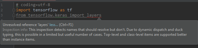

处理方法
改写为“from tensorflow.python.keras import layers”
导入包时，需要根据实际的具体位置进行导入。
确认TensorFlow中Keras的实际位置：“D:\DownLoadFiles\anaconda3\envs\mlcc\Lib\site-packages\tensorflow\python\keras\”。
实际上多了一层目录“python”，所以正确的导入方式为“from tensorflow.python.keras import layers”。

参考信息
https://stackoverflow.com/questions/47262955/how-to-import-keras-from-tf-keras-in-tensorflow

问题2：执行keras.utils.get_file()报错

问题描述
执行keras.utils.get_file("auto-mpg.data", "https://archive.ics.uci.edu/ml/machine-learning-databases/auto-mpg/auto-mpg.data")报错：

Downloading data from https://archive.ics.uci.edu/ml/machine-learning-databases/auto-mpg/auto-mpg.data
Traceback (most recent call last):
......
Exception: URL fetch failure on https://archive.ics.uci.edu/ml/machine-learning-databases/auto-mpg/auto-mpg.data: None -- [WinError 10060] A connection attempt failed because the connected party did not properly respond after a period of time, or established connection failed because connected host has failed to respond

处理方法
“网络”的原因，导致无法下载。手工下载，然后放置在当前目录，从当前目录地址导入数据文件。