python 招聘数据分析

导入包

import pandas as pd
import numpy as np
import matplotlib.pyplot as plt

读文件

df=pd.read_csv(r'C:\Users\MSI\Desktop\1.csv')

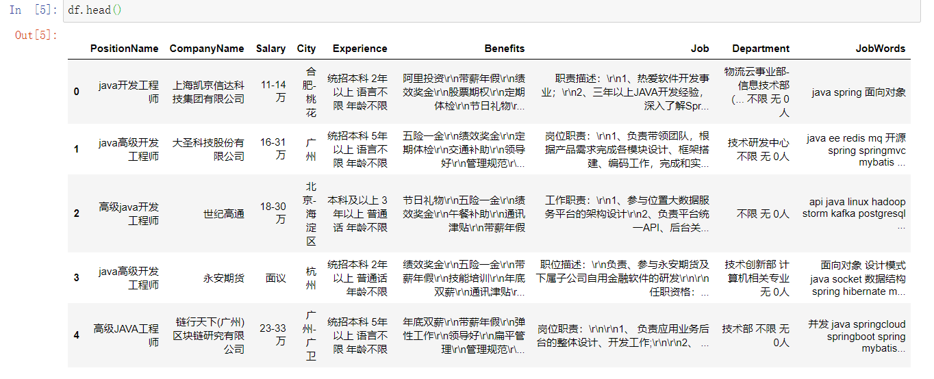
查看数据

df.head()

查看基本信息

df.info()

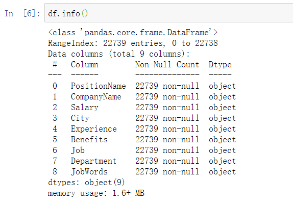
一共有九个字段，22739条数据，数据全为字符串，不存在数据为空的情况，因此不需要进行对缺少数据的处理

对重复数据进行处理，删除职位和公司重复值

df.drop_duplicates(['PositionName','CompanyName'],keep='first', inplace=True)

查看处理后的信息

df.info()

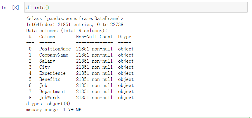
剩余21851条记录

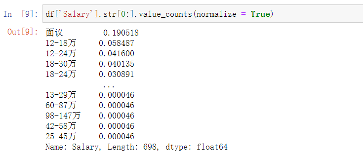
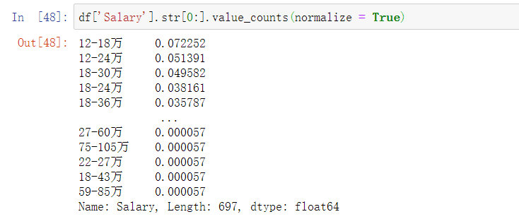
查看薪资的分布的频率，发现面议有较大的比重

df['Salary'].str[0:].value_counts(normalize = True)

自定义函数drops，删除薪资中的面议

def drops(col, tag):
    df.drop(df[df[col].str.contains(tag)].index, inplace=True)
drops('Salary', '面议')

自定义函数cutWord求平均薪资

def cutWord(word,method):
    position=word.find("-")
    length = len(word)
    if position != -1:
        bottomSalary = word[:position]
        topSalary = word[position + 1:length - 1]
    if method == 'bottom':
        return bottomSalary
    else:
        return topSalary

df['topSalary']=df.Salary.apply(cutWord,method='top')
df['bottomSalary']=df.Salary.apply(cutWord,method='bottom')

df.topSalary=df.topSalary.astype("int")
df.bottomSalary=df.bottomSalary.astype("int")

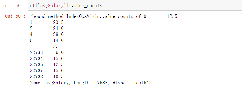
df['avgSalary']=df.apply(lambda x:(x.bottomSalary+x.topSalary)/2,axis=1)

df['avgSalary'].value_counts

由于各个仅统计各个省份，但所给数据中含有地级市及区等，因此对数据进行处理，仅保留省份/直辖市

自定义函数newCity

def newCity(city):
    if(len(str(city))>2):
        newcity = city[:2]
    else:
        newcity=city
    return newcity

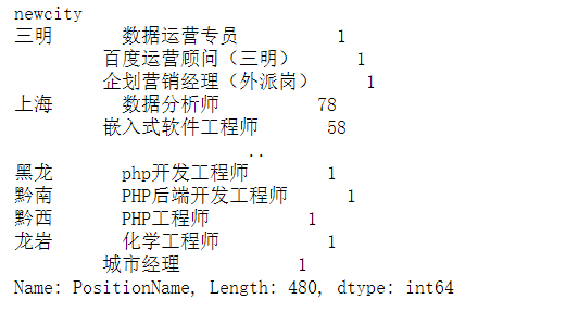
df['newcity']=df.City.apply(newCity)

数据基本处理完成，保存为df_clean

df_clean = df[["PositionName", "CompanyName", "newcity", "Experience", "JobWords", "avgSalary"]]
df_clean.head()

查看数据的描述性信息

print(df_clean.describe())

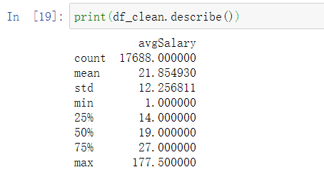
平均薪资：21.85W，中位数：19W，最高：177.5W

薪资分布情况图

plt.rcParams['font.sans-serif']=['SimHei']
df_clean.avgSalary.hist(bins=20)
plt.show()

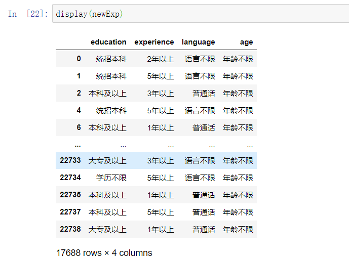
分割experience，不知道为什么这里分割了八个出来，我就定义了8列。不太懂我觉的这里应该四列才对,8列弄出来之后再把多的删了

info_split=df_clean['Experience'].str.split(' ',expand=True)
info_split.columns=['education','experience','language','age','1','2','3','4']

newExp=info_split.drop(['1','2','3','4'],axis=1)

display(newExp)

display(df_clean)

然后把两个二维表进行链接，再保存为new_df，最开始是链接之后删除experience，但是不知道为什么链接之后删除newcity就变成了city，之前的city白处理了。然后就直接保存了

newDF=pd.concat([df_clean, newExp], axis=1)

new_df = newDF[["PositionName", "CompanyName", "newcity",'education','experience','language','age' , "JobWords", "avgSalary"]]

display(new_df)

转换分类数据，这里发现本科有两个，然后其他数据不是很直观，后续有对这个数据进行了处理

new_df.education.astype('category')

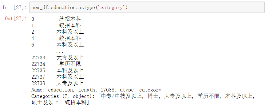
自定义newEdu处理教育水平，写的有点复杂，之前的写法不知道为什么最后的结构只剩下本科和硕士。

def newEdu(education):
    if education == "硕士及以上":
        new_edu = "硕士"
    elif education == "统招本科":
        new_edu = "本科"
    elif education == "本科及以上":
        new_edu = "本科"
    elif education== "学历不限":
        new_edu = "不限"
    elif education== "大专及以上":
        new_edu = "大专"
    elif education == "中专/中技及以上":
        new_edu = "中专"
    else:
        new_edu="博士"
    return new_edu

new_df['new_edu'] = new_df.education.apply(newEdu)

new_df.new_edu.astype('category')

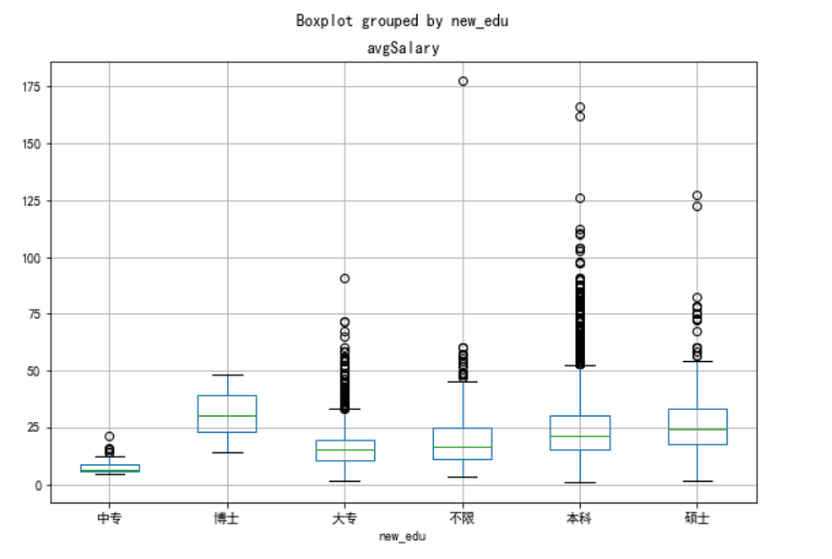
选用线箱进行比较。其最大的优点就是不受异常值的影响，可以以一种相对稳定的方式描述数据的平均水平、波动程度和异常值分布情况。

new_df.new_edu=new_df.new_edu.astype('category')
new_df.new_edu.cat.set_categories(["中专", "博士", "大专", "不限", "本科", "硕士", ],inplace=True)
ax=new_df.boxplot(column='avgSalary',by='new_edu',figsize=(9,6))

print(new_df.groupby(new_df.new_edu).avgSalary.mean().sort_values(ascending=False))

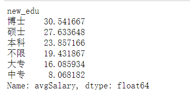
如图1，本科中位数薪资高于硕士生，容易误以为本科薪资高于硕士生，但同时结合图2，可见硕士生的平均薪资水平远高于本科生，由此可知，学历越高，薪资越高，知识改变命运。

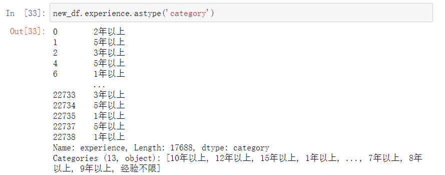
转化数据类型（工作年限）创建线箱进行比较

new_df.experience.astype('category')

new_df.boxplot(column='avgSalary',by='experience',figsize=(9,6))

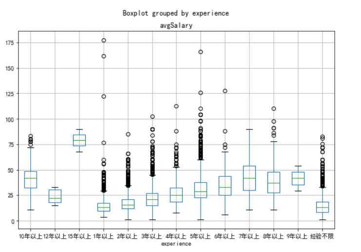
工作年限和薪资的比较

print(new_df.groupby(new_df.experience).avgSalary.mean().sort_values(ascending=False))

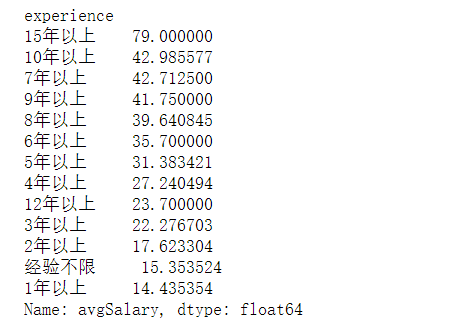
薪资与工作年限有很大关系，但优秀员工薪资明显超越年限限制。

北京和上海这两座城市，学历对薪资的影响

df_sz_bj=new_df[new_df['newcity'].isin(['上海','北京'])]
df_sz_bj.boxplot(column='avgSalary',by=['new_edu','newcity'],figsize=[14,6])
plt.show()

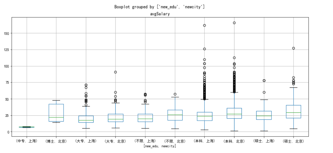
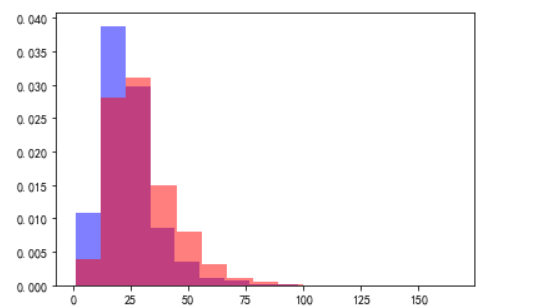
薪资与工作区域有很大关系，北京薪资不管什么学历都高于同等学历的薪资状况

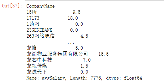
不同城市，招聘数据分析需求前五的公司

自定义了函数topN，将传入的数据计数，并且从大到小返回前五的数据。然后以newcity聚合分组，因为求的是前5的公司，所以对CompanyName调用topN函数。

new_df.groupby('CompanyName').avgSalary.agg(lambda x:max(x)-min(x))

def topN(df,n=5):
    counts=df.value_counts()
    return counts.sort_values(ascending=False)[:n]

print(new_df.groupby('newcity').CompanyName.apply(topN))

职位需求的前五，以计算机行业为主

print(new_df.groupby('newcity').PositionName.apply(topN))

将上海和北京的薪资数据以直方图的形式进行对比

plt.hist(x=new_df[new_df.newcity=='上海'].avgSalary,
         bins=15,
         density=1,
         facecolor='blue',
         alpha=0.5)
plt.hist(x=new_df[new_df.newcity=='北京'].avgSalary,
         bins=15,
         density=1,
         facecolor='red',
         alpha=0.5)
plt.show()

做一个所需要做的工作的词云，先下载wordcloud库

在anaconda下载第三方库还挺麻烦的，镜像还不能用，只能下载之后导包

查看数据进行处理

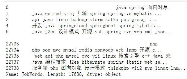
print(new_df.JobWords)

重置索引然后作词云

df_word_counts=df_word.unstack().dropna().reset_index().groupby('level_0').count()

from wordcloud import WordCloud
df_word_counts.index=df_word_counts.index.str.replace("'","")

wc=WordCloud(font_path=r'C:\Windows\Fonts\FZSTK.TTF',width=900,height=400,background_color='white')
fig,ax=plt.subplots(figsize=(20,15))
wc.fit_words(df_word_counts.level_1)
ax=plt.imshow(wc)
plt.axis('off')
plt.show()

上图可见对统计分析，数学，英语和office使用还是有一定的要求。

完整代码

#!/usr/bin/env python
# coding: utf-8

import pandas as pd
import numpy as np
import matplotlib.pyplot as plt

df=pd.read_csv(r'C:\Users\MSI\Desktop\1.csv')

df.head()

df.info()

df.drop_duplicates(['PositionName','CompanyName'],keep='first', inplace=True)

df.info()

df['Salary'].str[0:].value_counts(normalize = True)

def drops(col, tag):
    df.drop(df[df[col].str.contains(tag)].index, inplace=True)

drops('Salary', '面议')

df['Salary'].str[0:].value_counts(normalize = True)

def cutWord(word,method):
    position=word.find("-")
    length = len(word)
    if position != -1:
        bottomSalary = word[:position]
        topSalary = word[position + 1:length - 1]
    if method == 'bottom':
        return bottomSalary
    else:
        return topSalary

df['topSalary']=df.Salary.apply(cutWord,method='top')
df['bottomSalary']=df.Salary.apply(cutWord,method='bottom')

df.topSalary=df.topSalary.astype("int")
df.bottomSalary=df.bottomSalary.astype("int")

df['avgSalary']=df.apply(lambda x:(x.bottomSalary+x.topSalary)/2,axis=1)

df['avgSalary'].value_counts

def newCity(city):
    if(len(str(city))>2):
        newcity = city[:2]
    else:
        newcity=city
    return newcity

df['newcity']=df.City.apply(newCity)

df_clean = df[["PositionName", "CompanyName", "newcity", "Experience", "JobWords", "avgSalary"]]
df_clean.head()

print(df_clean.describe())

plt.rcParams['font.sans-serif']=['SimHei']
df_clean.avgSalary.hist(bins=20)
plt.show()

info_split=df_clean['Experience'].str.split(' ',expand=True)
info_split.columns=['education','experience','language','age','1','2','3','4']

newExp=info_split.drop(['1','2','3','4'],axis=1)

display(newExp)

display(df_clean)

newDF=pd.concat([df_clean, newExp], axis=1)

new_df = newDF[["PositionName", "CompanyName", "newcity",'education','experience','language','age' , "JobWords", "avgSalary"]]

display(new_df)

new_df.education.astype('category')

def newEdu(education):
    if education == "硕士及以上":
        new_edu = "硕士"
    elif education == "统招本科":
        new_edu = "本科"
    elif education == "本科及以上":
        new_edu = "本科"
    elif education== "学历不限":
        new_edu = "不限"
    elif education== "大专及以上":
        new_edu = "大专"
    elif education == "中专/中技及以上":
        new_edu = "中专"
    else:
        new_edu="博士"
    return new_edu

new_df['new_edu'] = new_df.education.apply(newEdu)

new_df.new_edu.astype('category')

new_df.new_edu=new_df.new_edu.astype('category')
new_df.new_edu.cat.set_categories(["中专", "博士", "大专", "不限", "本科", "硕士", ],inplace=True)
ax=new_df.boxplot(column='avgSalary',by='new_edu',figsize=(9,6))

print(new_df.groupby(new_df.new_edu).avgSalary.mean().sort_values(ascending=False))

new_df.experience.astype('category')

new_df.boxplot(column='avgSalary',by='experience',figsize=(9,6))

print(new_df.groupby(new_df.experience).avgSalary.mean().sort_values(ascending=False))

df_sz_bj=new_df[new_df['newcity'].isin(['上海','北京'])]
df_sz_bj.boxplot(column='avgSalary',by=['new_edu','newcity'],figsize=[14,6])
plt.show()

new_df.groupby('CompanyName').avgSalary.agg(lambda x:max(x)-min(x))

def topN(df,n=5):
    counts=df.value_counts()
    return counts.sort_values(ascending=False)[:n]

print(new_df.groupby('newcity').CompanyName.apply(topN))

print(new_df.groupby('newcity').PositionName.apply(topN))

plt.hist(x=new_df[new_df.newcity=='上海'].avgSalary,
         bins=15,
         density=1,
         facecolor='blue',
         alpha=0.5)
plt.hist(x=new_df[new_df.newcity=='北京'].avgSalary,
         bins=15,
         density=1,
         facecolor='red',
         alpha=0.5)
plt.show()

print(new_df.JobWords)

df_word_counts=df_word.unstack().dropna().reset_index().groupby('level_0').count()

from wordcloud import WordCloud
df_word_counts.index=df_word_counts.index.str.replace("'","")

wc=WordCloud(font_path=r'C:\Windows\Fonts\FZSTK.TTF',width=900,height=400,background_color='white')
fig,ax=plt.subplots(figsize=(20,15))
wc.fit_words(df_word_counts.level_1)
ax=plt.imshow(wc)
plt.axis('off')
plt.show()

参考资料：

https://www.jianshu.com/p/1e1081ca13b5