SVM算法简单应用

第一部分：线性可分

通俗解释：可以用一条直线将两类分隔开来

一个简单的例子，直角坐标系中有三个点，A，B点为0类，C点为1类：

from sklearn import svm

# 三个点
x = [[1, 1], [2, 0], [2, 3]]
# 三个点所属类
y = [0, 0, 1]

clf = svm.SVC(kernel='linear')
clf.fit(x, y)

# 所有信息
print(clf)
# 支持向量
print(clf.support_vectors_)
# 支持向量在x中的索引
print(clf.support_)
# 支持向量在所属类中分别有几个
print(clf.n_support_)
# 预测（1，4）这个点所属分类，结果是1类
print(clf.predict([[1, 4]]))

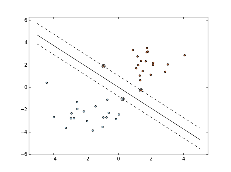
接下来多一些数据并画图观察下：

import numpy as np
import pylab as pl
from sklearn import svm

# 按正态分布随机取40个样本
# 前20个取[-2,-2]点附近样本，后20个取[2,2]点附近样本，再用np.r_拼接
X = np.r_[np.random.randn(20, 2) - [2, 2], np.random.randn(20, 2) + [2, 2]]
# 20个0类20个1类
Y = [0] * 20 + [1] * 20

# 调用sklearn的SVM
clf = svm.SVC(kernel='linear')
clf.fit(X, Y)

# 参数
w = clf.coef_[0]

'''
w_0x + w_1y +w_3=0方程转化为：
y = -(w_0/w_1) x + (w_3/w_1)
其中w_3=clf.intercept_[0]
'''

# 直线斜率
a = -w[0] / w[1]
# 取-5到5之间的一些浮点数
xx = np.linspace(-5, 5)
# 直线方程
yy = a * xx - (clf.intercept_[0]) / w[1]
# 取第一个支持向量
b = clf.support_vectors_[0]
# 下方直线方程（利用点斜式方程）
yy_down = a * xx + (b[1] - a * b[0])
# 取最后一个支持向量
b = clf.support_vectors_[-1]
# 上方直线方程（同理）
yy_up = a * xx + (b[1] - a * b[0])

# 画出三条直线
pl.plot(xx, yy, 'k-')
pl.plot(xx, yy_down, 'k--')
pl.plot(xx, yy_up, 'k--')

# 画出这些点
pl.scatter(clf.support_vectors_[:, 0], clf.support_vectors_[:, 1],
           s=80, facecolors='none')
pl.scatter(X[:, 0], X[:, 1], c=Y, cmap=pl.cm.Paired)

# 使坐标系的最大值和最小值与数据范围一致
pl.axis('tight')

# 展示
pl.show()

第二部分：线性不可分

不可以用一条直线分割开来的数据

方法：转换成高维度

人脸识别案例：

from __future__ import print_function
from time import time
import logging
import matplotlib.pyplot as plt
from sklearn.cross_validation import train_test_split
from sklearn.datasets import fetch_lfw_people
from sklearn.grid_search import GridSearchCV
from sklearn.metrics import classification_report
from sklearn.metrics import confusion_matrix
from sklearn.decomposition import RandomizedPCA
from sklearn.svm import SVC

# 打印日志
logging.basicConfig(level=logging.INFO, format='%(asctime)s %(message)s')
# 装载数据集
lfw_people = fetch_lfw_people(min_faces_per_person=70, resize=0.4)
# 处理图片相关信息
n_samples, h, w = lfw_people.images.shape
X = lfw_people.data
n_features = X.shape[1]
y = lfw_people.target
target_names = lfw_people.target_names
n_classes = target_names.shape[0]
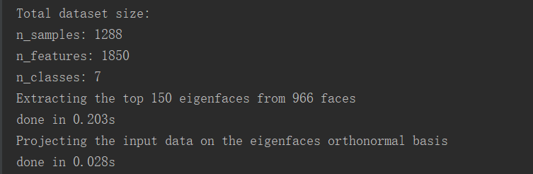
print("Total dataset size:")
print("n_samples: %d" % n_samples)
print("n_features: %d" % n_features)
print("n_classes: %d" % n_classes)

# 设置训练集和测试集
# 随机选取75%的数据作为训练样本
# 其余25%的数据作为测试样本
X_train, X_test, y_train, y_test = train_test_split(
    X, y, test_size=0.25)

# 降低维度（PCA算法）
n_components = 150

print("Extracting the top %d eigenfaces from %d faces"
      % (n_components, X_train.shape[0]))
t0 = time()
pca = RandomizedPCA(n_components=n_components, whiten=True).fit(X_train)
print("done in %0.3fs" % (time() - t0))

eigenfaces = pca.components_.reshape((n_components, h, w))

print("Projecting the input data on the eigenfaces orthonormal basis")
t0 = time()
X_train_pca = pca.transform(X_train)
X_test_pca = pca.transform(X_test)
print("done in %0.3fs" % (time() - t0))

# SVM算法
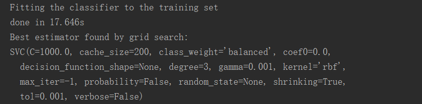
print("Fitting the classifier to the training set")
t0 = time()
param_grid = {'C': [1e3, 5e3, 1e4, 5e4, 1e5],
              'gamma': [0.0001, 0.0005, 0.001, 0.005, 0.01, 0.1], }
clf = GridSearchCV(SVC(kernel='rbf', class_weight='balanced'), param_grid)
clf = clf.fit(X_train_pca, y_train)
print("done in %0.3fs" % (time() - t0))
print("Best estimator found by grid search:")
print(clf.best_estimator_)

# 预测

print("Predicting people's names on the test set")
t0 = time()
y_pred = clf.predict(X_test_pca)
print("done in %0.3fs" % (time() - t0))

print(classification_report(y_test, y_pred, target_names=target_names))
print(confusion_matrix(y_test, y_pred, labels=range(n_classes)))

# 画图展示
def plot_gallery(images, titles, h, w, n_row=3, n_col=4):
    plt.figure(figsize=(1.8 * n_col, 2.4 * n_row))
    plt.subplots_adjust(bottom=0, left=.01, right=.99, top=.90, hspace=.35)
    for i in range(n_row * n_col):
        plt.subplot(n_row, n_col, i + 1)
        plt.imshow(images[i].reshape((h, w)), cmap=plt.cm.gray)
        plt.title(titles[i], size=12)
        plt.xticks(())
        plt.yticks(())

# 展示的每一张图标题（判断正误）
def title(y_pred, y_test, target_names, i):
    pred_name = target_names[y_pred[i]].rsplit(' ', 1)[-1]
    true_name = target_names[y_test[i]].rsplit(' ', 1)[-1]
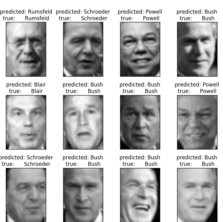
    return 'predicted: %s\ntrue:      %s' % (pred_name, true_name)

prediction_titles = [title(y_pred, y_test, target_names, i)
                     for i in range(y_pred.shape[0])]

# 原来的图片
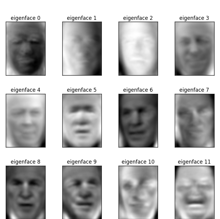
plot_gallery(X_test, prediction_titles, h, w)

eigenface_titles = ["eigenface %d" % i for i in range(eigenfaces.shape[0])]
# 提取人脸特征的图片
plot_gallery(eigenfaces, eigenface_titles, h, w)

plt.show()

数据相关信息：

PCA和SVM算法：

预测：

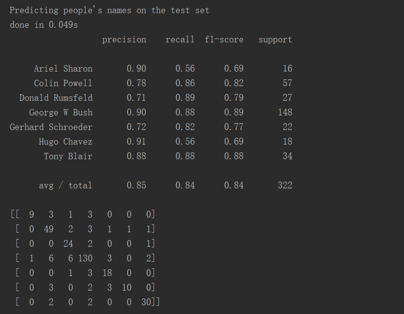
发现精确度达到85%，比较成功

观察矩阵：对角线代表预测与真实一致的个数

最后形象地看下：预测结果和真实基本一致

特征图：