CNN初步-1

Convolution:

 

个特征，则这时候把输入层的所有点都与隐含层节点连接，则需要学习10^6个参数，这样的话在使用BP算法时速度就明显慢了很多。

所以后面就发展到了局部连接网络，也就是说每个隐含层的节点只与一部分连续的输入点连接。这样的好处是模拟了人大脑皮层中视觉皮层不同位置只对局部区域有响应。局部连接网络在神经网络中的实现使用convolution的方法。它在神经网络中的理论基础是对于自然图像来说，因为它们具有稳定性，即图像中某个部分的统计特征和其它部位的相似，因此我们学习到的某个部位的特征也同样适用于其它部位。

下面具体看一个例子是怎样实现convolution的，假如对一张大图片Xlarge的数据集，r*c大小，则首先需要对这个数据集随机采样大小为a*b的小图片，然后用这些小图片patch进行学习（比如说sparse autoencoder），此时的隐含节点为k个。因此最终学习到的特征数为：

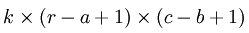
此时的convolution移动是有重叠的。

Formally, given some large  images x_large, we first train a sparse autoencoder on small  patches x_small sampled from these images, learning k features f = σ(W⁽¹⁾x_small + b⁽¹⁾) (where σ is the sigmoid function), given by the weights W⁽¹⁾ and biases b⁽¹⁾ from the visible units to the hidden units. For every  patch x_s in the large image, we compute f_s = σ(W⁽¹⁾x_s+ b⁽¹⁾), giving us f_convolved, a  array of convolved features.

总结：

convolution解决了训练输入特征过多的问题。采用小patch 采样训练，训练后的结果filter 再作用到所有图片区域。

Pooling：

个隐含层，则其需要训练的参数个数减小到了10^3，大大的减小特征提取过程的困难。但是此时同样出现了一个问题，即它的输出向量的维数变得很大，本来完全连接的网络输出只有100维的，现在的网络输出为89*89*100=792100维，大大的变大了，这对后面的分类器的设计同样带来了困难，所以pooling方法就出现了。

为什么pooling的方法可以工作呢？首先在前面的使用convolution时是利用了图像的stationarity特征，即不同部位的图像的统计特征是相同的，那么在使用convolution对图片中的某个局部部位计算时，得到的一个向量应该是对这个图像局部的一个特征，既然图像有stationarity特征，那么对这个得到的特征向量进行统计计算的话，所有的图像局部块应该也都能得到相似的结果。对convolution得到的结果进行统计计算过程就叫做pooling，由此可见pooling也是有效的。常见的pooling方法有max pooling和average pooling等。并且学习到的特征具有旋转不变性（这个原因暂时没能理解清楚）。

从上面的介绍可以简单的知道，convolution是为了解决前面无监督特征提取学习计算复杂度的问题，而pooling方法是为了后面有监督特征分类器学习的，也是为了减小需要训练的系统参数（当然这是在普遍例子中的理解，也就是说我们采用无监督的方法提取目标的特征，而采用有监督的方法来训练分类器）。

总结：

convolution解决了输入层参数多问题，但是输出特征太多，pooling解决了这一问题。

来自 <http://www.cnblogs.com/tornadomeet/archive/2013/03/25/2980766.html>

http://deeplearning.stanford.edu/wiki/index.php/Feature_extraction_using_convolution

http://deeplearning.stanford.edu/wiki/index.php/Pooling

http://deeplearning.net/tutorial/lenet.html

先看下 convolution

import theano

from theano import tensor as T

from theano.tensor.nnet import conv

import numpy

rng = numpy.random.RandomState(23455)

# instantiate 4D tensor for input

input = T.tensor4(name='input')

# initialize shared variable for weights.

w_shp = (2, 3, 9, 9)

w_bound = numpy.sqrt(3 * 9 * 9)

W = theano.shared( numpy.asarray(

rng.uniform(

low=-1.0 / w_bound,

high=1.0 / w_bound,

size=w_shp),

dtype=input.dtype), name ='W')

# initialize shared variable for bias (1D tensor) with random values

# IMPORTANT: biases are usually initialized to zero. However in this

# particular application, we simply apply the convolutional layer to

# an image without learning the parameters. We therefore initialize

# them to random values to "simulate" learning.

b_shp = (2,)

b = theano.shared(numpy.asarray(

rng.uniform(low=-.5, high=.5, size=b_shp),

dtype=input.dtype), name ='b')

# build symbolic expression that computes the convolution of input with filters in w

conv_out = conv.conv2d(input, W)

# build symbolic expression to add bias and apply activation function, i.e. produce neural net layer output

# A few words on ``dimshuffle`` :

# ``dimshuffle`` is a powerful tool in reshaping a tensor;

# what it allows you to do is to shuffle dimension around

# but also to insert new ones along which the tensor will be

# broadcastable;

# dimshuffle('x', 2, 'x', 0, 1)

# This will work on 3d tensors with no broadcastable

# dimensions. The first dimension will be broadcastable,

# then we will have the third dimension of the input tensor as

# the second of the resulting tensor, etc. If the tensor has

# shape (20, 30, 40), the resulting tensor will have dimensions

# (1, 40, 1, 20, 30). (AxBxC tensor is mapped to 1xCx1xAxB tensor)

# More examples:

# dimshuffle('x') -> make a 0d (scalar) into a 1d vector

# dimshuffle(0, 1) -> identity

# dimshuffle(1, 0) -> inverts the first and second dimensions

# dimshuffle('x', 0) -> make a row out of a 1d vector (N to 1xN)

# dimshuffle(0, 'x') -> make a column out of a 1d vector (N to Nx1)

# dimshuffle(2, 0, 1) -> AxBxC to CxAxB

# dimshuffle(0, 'x', 1) -> AxB to Ax1xB

# dimshuffle(1, 'x', 0) -> AxB to Bx1xA

output = T.nnet.sigmoid(conv_out + b.dimshuffle('x', 0, 'x', 'x')) #(1,2,1,1)

# create theano function to compute filtered images

f = theano.function([input], output)

import sys

import numpy

import pylab

from PIL import Image

# open random image of dimensions 639x516

img = Image.open(open(sys.argv[1]))

# dimensions are (height, width, channel)

img = numpy.asarray(img, dtype='float64') / 256.

# put image in 4D tensor of shape (1, 3, height, width)

img_ = img.transpose(2, 0, 1).reshape(1, 3, img.shape[0], img.shape[1])

filtered_img = f(img_)

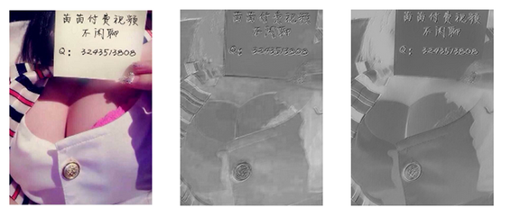
# plot original image and first and second components of output

pylab.subplot(1, 3, 1); pylab.axis('off'); pylab.imshow(img)

pylab.gray();

# recall that the convOp output (filtered image) is actually a "minibatch",

# of size 1 here, so we take index 0 in the first dimension:

pylab.subplot(1, 3, 2); pylab.axis('off'); pylab.imshow(filtered_img[0, 0, :, :])

pylab.subplot(1, 3, 3); pylab.axis('off'); pylab.imshow(filtered_img[0, 1, :, :])

#pylab.show()

from gezi import show

show()

狼的例子

img.shape

Out[57]: (639, 516, 3)

In [58]: img_.shape

Out[58]: (1, 3, 639, 516) #conv输入数据

filtered_img.shape

Out[56]: (1, 2, 631, 508)

这个刚好 因为w_shp = (2, 3, 9, 9)

In [66]: rng.uniform(low=-1.0 / w_bound, high=1.0 / w_bound, size=w_shp).shape

Out[66]: (2, 3, 9, 9)

采用的是9*9的patch

所以处理后

是 (639 - 9 + 1) * (516 - 9 + 1) 631 * 508

参考这个

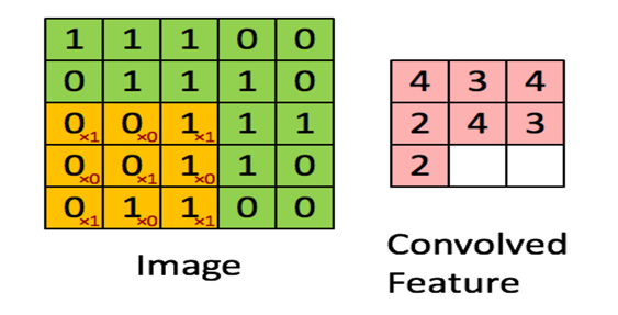
结果刚好类似一个edge detector ，用一个非狼的例子