MATLAB 颜色图函数（imagesc/scatter/polarPcolor/pcolor）

2维的热度图 imagesc

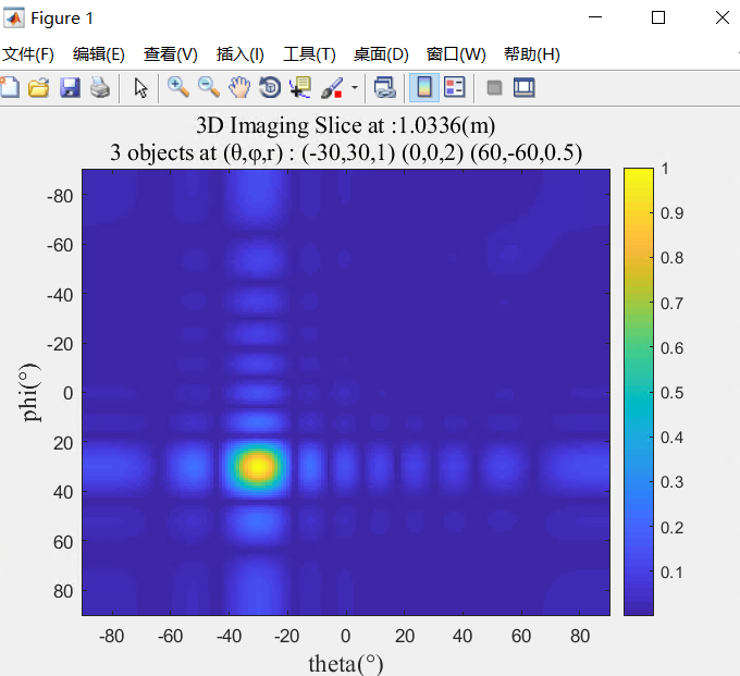
imagesc（x, y, z），x和y分别是横纵坐标，z为值，表示颜色

 imagesc(theta,phi,slc); colorbar
 xlabel('theta(°)','fontname','Times New Roman','FontSize',);
 ylabel('phi(°)','fontname','Times New Roman','FontSize',);
 sta = '3 objects at (θ,φ,r) : (-30,30,1) (0,0,2) (60,-60,0.5)';
 str=sprintf(strcat('3D Imaging Slice at :', num2str(d_max*D/N), '(m)', '\n',sta));
 title(str, 'fontname','Times New Roman','Color','k','FontSize',);
 grid on

其中，colorbar的坐标值调整：caxis([0 1]);

colormap的色系调整：colormap hot

3维散点图 scatter

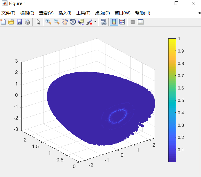
 scatter3(x,y,z,,c,'filled');
 % axis([-(R+) (R+) -(R+) (R+)  (h+)]);
 colorbar

2维 极坐标热度图 polarPcolor

polarPcolor(R_axis, theta, value)，前两个为半径方向坐标轴和圆心角坐标轴，value为值，用颜色表示

 [fig, clr] = polarPcolor(R_axis, theta, x_d_th, 'labelR','range (m)','Ncircles', ,'Nspokes',);
 colormap hot
 % caxis([ ]);

其中polarPcolor代码如下：

 function [varargout] = polarPcolor(R,theta,Z,varargin)
 % [h,c] = polarPcolor1(R,theta,Z,varargin) is a pseudocolor plot of matrix
 % Z for a vector radius R and a vector angle theta.
 % The elements of Z specify the color in each cell of the
 % plot. The goal is to apply pcolor function with a polar grid, which
 % provides a better visualization than a cartesian grid.
 %
 %% Syntax
 %
 % [h,c] = polarPcolor(R,theta,Z)
 % [h,c] = polarPcolor(R,theta,Z,'Ncircles',)
 % [h,c] = polarPcolor(R,theta,Z,'Nspokes',)
 % [h,c] = polarPcolor(R,theta,Z,'Nspokes',,'colBar',)
 % [h,c] = polarPcolor(R,theta,Z,'Nspokes',,'labelR','r (km)')
 %
 % INPUT
 %    * R :
 %        - type: float
 %        - size: [ x Nrr ] where Nrr = numel(R).
 %        - dimension: radial distance.
 %    * theta :
 %        - type: float
 %        - size: [ x Ntheta ] where Ntheta = numel(theta).
 %        - dimension: azimuth or elevation angle (deg).
 %        - N.B.: The zero is defined with respect to the North.
 %    * Z :
 %        - type: float
 %        - size: [Ntheta x Nrr]
 %        - dimension: user's defined .
 %    * varargin:
 %        - Ncircles: number  of circles for the grid definition.
 %        - Nspokes: number of spokes for the grid definition.
 %        - colBar: display the colorbar or not.
 %        - labelR: legend for R.
 %
 %
 % OUTPUT
 % h: returns a handle to a SURFACE object.
 % c: returns a handle to a COLORBAR object.
 %
 %% Examples
 % R = linspace(,,);
 % theta = linspace(,,);
 % Z = linspace(,,)'*linspace(0,10,100);
 % figure
 % polarPcolor(R,theta,Z,'Ncircles',)
 %
 %% Author
 % Etienne Cheynet, University of Stavanger, Norway. //
 % see also pcolor
 % 

 %%  InputParseer
 p = inputParser();
 p.CaseSensitive = false;
 p.addOptional('Ncircles',);
 p.addOptional('Nspokes',);
 p.addOptional('labelR','');
 p.addOptional('colBar',);
 p.parse(varargin{:});

 Ncircles = p.Results.Ncircles ;
 Nspokes = p.Results.Nspokes ;
 labelR = p.Results.labelR ;
 colBar = p.Results.colBar ;
 %% Preliminary checks
 % case where dimension is reversed
 Nrr = numel(R);
 Noo = numel(theta);
 if isequal(size(Z),[Noo,Nrr]),
     Z=Z';
 end

 % case where dimension of Z is not compatible with theta and R
 if ~isequal(size(Z),[Nrr,Noo])
     fprintf('\n')
     fprintf([ 'Size of Z is : [',num2str(size(Z)),'] \n']);
     fprintf([ 'Size of R is : [',num2str(size(R)),'] \n']);
     fprintf([ 'Size of theta is : [',num2str(size(theta)),'] \n\n']);
     error(' dimension of Z does not agree with dimension of R and Theta')
 end
 %% data plot
 rMin = min(R);
 rMax = max(R);
 thetaMin=min(theta);
 thetaMax =max(theta);
 % Definition of the mesh
 Rrange = rMax - rMin; % get the range for the radius
 rNorm = R/Rrange; %normalized radius [,]
 % get hold state
 cax = newplot;
 % transform data in polar coordinates to Cartesian coordinates.
 YY = (rNorm)'*cosd(theta);
 XX = (rNorm)'*sind(theta);
 % plot data on top of grid
 h = pcolor(XX,YY,Z,'parent',cax);
 shading flat
 set(cax,'dataaspectratio',[  ]);axis off;
 if ~ishold(cax);
     % make a radial grid
     hold(cax,'on')
     % Draw circles and spokes
     createSpokes(thetaMin,thetaMax,Ncircles,Nspokes);
     createCircles(rMin,rMax,thetaMin,thetaMax,Ncircles,Nspokes)
 end

 %% PLot colorbar if specified
 if colBar==,
     c =colorbar('location','WestOutside');
     caxis([quantile(Z(:),0.01),quantile(Z(:),0.99)])
 else
     c = [];
 end

 %% Outputs
 nargoutchk(,)
 if nargout==,
     varargout{}=h;
 elseif nargout==,
     varargout{}=h;
     varargout{}=c;
 end

 %%%%%%%%%%%%%%%%%%%%%%%%%%%%%%%%%%%%%%%%%%%%%%%%%%%%%%%%%%%%%%%%%%%%%%%%%%%
 % Nested functions
 %%%%%%%%%%%%%%%%%%%%%%%%%%%%%%%%%%%%%%%%%%%%%%%%%%%%%%%%%%%%%%%%%%%%%%%%%%%
     function createSpokes(thetaMin,thetaMax,Ncircles,Nspokes)

         circleMesh = linspace(rMin,rMax,Ncircles);
         spokeMesh = linspace(thetaMin,thetaMax,Nspokes);
         contour = abs((circleMesh - circleMesh())/Rrange+R()/Rrange);
         cost = cosd(-spokeMesh); % the zero angle is aligned with North
         sint = sind(-spokeMesh); % the zero angle is aligned with North
         for kk = :Nspokes
             plot(cost(kk)*contour,sint(kk)*contour,'k:',...
                 'handlevisibility','off');
             % plot graduations of angles
             % avoid superimposition of  and
             if and(thetaMin==,thetaMax == ),
                 if spokeMesh(kk)<,

                     text(1.05.*contour(end).*cost(kk),...
                         1.05.*contour(end).*sint(kk),...
                         [num2str(spokeMesh(kk),),char()],...
                         'horiz', 'center', 'vert', 'middle');
                 end
             else
                 text(1.05.*contour(end).*cost(kk),...
                     1.05.*contour(end).*sint(kk),...
                     [num2str(spokeMesh(kk),),char()],...
                     'horiz', 'center', 'vert', 'middle');
             end

         end
     end
     function createCircles(rMin,rMax,thetaMin,thetaMax,Ncircles,Nspokes)

         % define the grid in polar coordinates
         angleGrid = linspace(-thetaMin,-thetaMax,);
         xGrid = cosd(angleGrid);
         yGrid = sind(angleGrid);
         circleMesh = linspace(rMin,rMax,Ncircles);
         spokeMesh = linspace(thetaMin,thetaMax,Nspokes);
         contour = abs((circleMesh - circleMesh())/Rrange+R()/Rrange);
         % plot circles
         for kk=:length(contour)
             plot(xGrid*contour(kk), yGrid*contour(kk),'k:');
         end
         % radius tick label
         for kk=:Ncircles

             position = 0.51.*(spokeMesh(min(Nspokes,round(Ncircles/)))+...
                 spokeMesh(min(Nspokes,+round(Ncircles/))));

             if abs(round(position)) ==,
                 % radial graduations
                 text((contour(kk)).*cosd(-position),...
                     (0.1+contour(kk)).*sind(-position),...
                     num2str(circleMesh(kk),),'verticalalignment','BaseLine',...
                     'horizontalAlignment', 'center',...
                     'handlevisibility','off','parent',cax);

                 % annotate spokes
                 text(contour(end).*0.6.*cosd(-position),...
                     0.07+contour(end).*0.6.*sind(-position),...
                     [labelR],'verticalalignment','bottom',...
                     'horizontalAlignment', 'right',...
                     'handlevisibility','off','parent',cax);
             else
                 % radial graduations
                 text((contour(kk)).*cosd(-position),...
                     (contour(kk)).*sind(-position),...
                     num2str(circleMesh(kk),),'verticalalignment','BaseLine',...
                     'horizontalAlignment', 'right',...
                     'handlevisibility','off','parent',cax);

                 % annotate spokes
                 text(contour(end).*0.6.*cosd(-position),...
                     contour(end).*0.6.*sind(-position),...
                     [labelR],'verticalalignment','bottom',...
                     'horizontalAlignment', 'right',...
                     'handlevisibility','off','parent',cax);
             end
         end

     end
 end

再贴一个示例代码：

 %% Examples
 % The following examples illustrate the application of the function
 % polarPcolor
 clearvars;close all;clc;

 %% Minimalist example
 % Assuming that a remote sensor is measuring the wind field for a radial
 % distance ranging from  to  m. The scanning azimuth is oriented from
 % North ( deg) to North-North-East (  deg):
 R = linspace(,,)./; % (distance in km)
 Az = linspace(,,); % in degrees
 [~,~,windSpeed] = peaks(); % radial wind speed
 figure()
 [h,c]=polarPcolor(R,Az,windSpeed);

 %% Example with options
 %  We want to have  circles and  spokes, and to give a label to the
 %  radial coordinate

 figure()
 [~,c]=polarPcolor(R,Az,windSpeed,'labelR','r (km)','Ncircles',,'Nspokes',);
 ylabel(c,' radial wind speed (m/s)');
 set(gcf,'color','w')
 %% Dealing with outliers
 % We introduce outliers in the wind velocity data. These outliers
 % are represented as wind speed sample with a value of  m/s. These
 % corresponds to unrealistic data that need to be ignored. To avoid bad
 % scaling of the colorbar, the function polarPcolor uses the function caxis
 % combined to the function quantile to keep the colorbar properly scaled:
 % caxis([quantile(Z(:),0.01),quantile(Z(:),0.99)])

 windSpeed(::end,::end)=;

 figure()
 [~,c]=polarPcolor(R,Az,windSpeed);
 ylabel(c,' radial wind speed (m/s)');
 set(gcf,'color','w')

 %% polarPcolor without colorbar
 % The colorbar is activated by default. It is possible to remove it by
 % using the option 'colBar'. When the colorbar is desactivated, the
 % outliers are not "removed" and bad scaling is clearly visible:

 figure()
 polarPcolor(R,Az,windSpeed,'colBar',) ;

 %% Different geometry
 N = ;
 R = linspace(,,N)./; % (distance in km)
 Az = linspace(,,N); % in degrees
 [~,~,windSpeed] = peaks(N); % radial wind speed
 figure()
 [~,c]= polarPcolor(R,Az,windSpeed);
 ylabel(c,' radial wind speed (m/s)');
 set(gcf,'color','w')
 %% Different geometry
 N = ;
 R = linspace(,,N)./; % (distance in km)
 Az = linspace(,,N); % in degrees
 [~,~,windSpeed] = peaks(N); % radial wind speed
 figure()
 [~,c]= polarPcolor(R,Az,windSpeed,'Ncircles',);
 location = 'NorthOutside';
 ylabel(c,' radial wind speed (m/s)');
 set(c,'location',location);
 set(gcf,'color','w')