【原】Coursera—Andrew Ng机器学习—编程作业 Programming Exercise 4

课程笔记

Coursera—Andrew Ng机器学习—课程笔记 Lecture 9_Neural Networks learning

作业说明

Exercise 4，Week 5，实现反向传播 backpropagation神经网络算法，对图片中手写数字 0-9 进行识别。

数据集 ：ex4data1.mat。手写数字图片数据，5000个样例。每张图片20px * 20px，也就是一共400个特征。数据集X维度为5000 * 400

　　　 ex4weights.mat。神经网络每一层的权重。

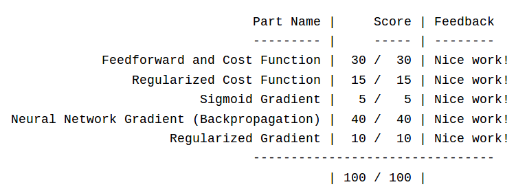
文件清单

ex4.m- Octave/MATLAB script that steps you through the exercise
ex4data1.mat- Training set of hand-written digits
ex4weights.mat- Neural network parameters for exercise 4
submit.m- Submission script that sends your solutions to our servers
displayData.m- Function to help visualize the dataset
fmincg.m- Function minimization routine (similar to fminunc)
sigmoid.m- Sigmoid function
computeNumericalGradient.m- Numerically compute gradients
checkNNGradients.m- Function to help check your gradients
debugInitializeWeights.m- Function for initializing weights
predict.m- Neural network prediction function
[*] sigmoidGradient.m- Compute the gradient of the sigmoid function
[*] randInitializeWeights.m- Randomly initialize weights
[*] nnCostFunction.m- Neural network cost function

　　* 为必须要完成的

结论

和上一周的作业一样。因为Octave里数组下标从1开始。所以这里将分类结果0用10替代。预测结果中的1-10代表图片数字为1,2,3,4,5,6,7,8,9,0

矩阵运算 tricky 的地方在于维度对应，哪里需要转置很关键。

1 神经网络

1.1 数据可视化

在数据集X里随机选择100个数字，绘制图像

displayData.m：

function [h, display_array] = displayData(X, example_width)

%DISPLAYDATA Display 2D data in a nice grid

%   [h, display_array] = DISPLAYDATA(X, example_width) displays 2D data

%   stored in X in a nice grid. It returns the figure handle h and the

%   displayed array if requested.

% Set example_width automatically if not passed in

if ~exist('example_width', 'var') || isempty(example_width)

    example_width = round(sqrt(size(X, 2)));

end

% Gray Image

colormap(gray);

% Compute rows, cols

[m n] = size(X);

example_height = (n / example_width);

% Compute number of items to display

display_rows = floor(sqrt(m));

display_cols = ceil(m / display_rows);

% Between images padding

pad = 1;

% Setup blank display

display_array = - ones(pad + display_rows * (example_height + pad), ...

                       pad + display_cols * (example_width + pad));

% Copy each example into a patch on the display array

curr_ex = 1;

for j = 1:display_rows

    for i = 1:display_cols

        if curr_ex > m,

            break;

        end

        % Copy the patch

        % Get the max value of the patch

        max_val = max(abs(X(curr_ex, :)));

        display_array(pad + (j - 1) * (example_height + pad) + (1:example_height), ...

                      pad + (i - 1) * (example_width + pad) + (1:example_width)) = ...

                        reshape(X(curr_ex, :), example_height, example_width) / max_val;

        curr_ex = curr_ex + 1;

    end

    if curr_ex > m,

        break;

    end

end

% Display Image

h = imagesc(display_array, [-1 1]);

% Do not show axis

axis image off

drawnow;

end

ex4.m里的调用

load('ex4data1.mat');

m = size(X, );

% Randomly select  data points to display

sel = randperm(size(X, ));

sel = sel(:);

displayData(X(sel, :));

运行效果如下：

1.2 模型表示

ex4.m 里载入已经调好的权重矩阵weight。

% Load saved matrices from file

load('ex4weights.mat');

% The matrices Theta1 and Theta2 will now be in your workspace

% Theta1 has size 25 x 401

% Theta2 has size 10 x

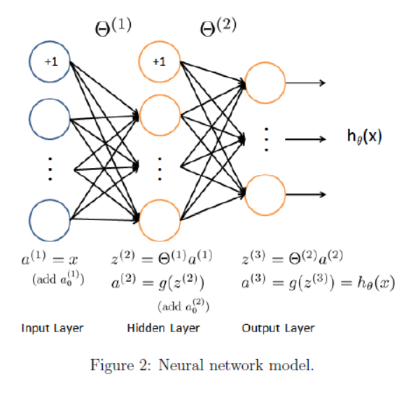
这里g(z) 使用 sigmoid 函数。

神经网络中，从上到下的每个原点是 feature 特征 x0, x1, x2...，不是实例。计算过程其实就是 feature 一层一层映射的过程。一层转换之后，feature可能变多、也可能变少。下一层 i+1层 feature 的个数是通过权重矩阵里当前 θ⁽ⁱ⁾ 的 row 行数来控制。

两层权重 θ 已经在 ex4weights.mat 里给出。从a1映射到a2权重矩阵 θ₁为 25 * 401，从a2映射到a3权重矩阵 θ₂为10 * 26。因为最后有10个分类。（这意味着运算的时候要注意转置）

1.3 前馈神经网络和代价函数

首先完成不包含正则项的代价函数，公式如下：

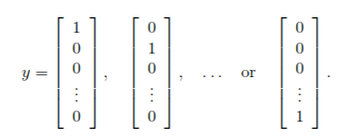
注意，和之前不同的是：由于y是范围0-9的数字，计算之前需要转换为下面这种向量的形式：

代码为：

% convert y（-） to vector

c = :num_labels;

yt = zeros(m,num_labels);

for i = :m

    yt(i,:) = (c==y(i));

end

nnCostFunction.m 计算代价函数的代码如下：

% compute h(x)

a1 = [ones(m, ) X];    %5000x401

a2 = sigmoid(a1 * Theta1');  %5000x401乘以401x25得到5000x25。即把401个feature映射到25

a2 = [ones(m, ) a2];    %5000x26

hx = sigmoid(a2 * Theta2');  %5000x26乘以26x10得到5000x10。即把26个feature映射到10

% first term

part1 = -yt.*log(hx);

% second term

part2 = (-yt).*log(-hx);

% compute J

J =  / m * sum(sum(part1 - part2));

需要注意的是，上一次作业里逻辑回归的代价函数计算使用的是矩阵相乘的方式

part1 = -yt' * log(hx);  part2 = (1-yt') * log(1-hx);

而这里神经网络的公式中有两层求和，需要使用 “矩阵点乘，sum，再sum” 的方式计算。如果使用矩阵相乘省略一层sum，结果会出错。

1.4 正则化的代价函数

给神经网络中的代价函数加上正则项，公式如下：

nnCostFunction.m 代码如下：

% convert y（-） to vector

c = :num_labels;

yt = zeros(m,num_labels);

for i = :m

    yt(i,:) = (c==y(i));

end

% compute h(x)

a1 = [ones(m, ) X];    %5000x401

a2 = sigmoid(a1 * Theta1');  %5000x401乘以401x25得到5000x25。即把401个feature映射到25

a2 = [ones(m, ) a2];    %5000x26

hx = sigmoid(a2 * Theta2');  %5000x26乘以26x10得到5000x10。即把26个feature映射到10

% first term

part1 = -yt.*log(hx);

% second term

part2 = (-yt).*log(-hx);

% regularization term

regTerm = lambda /  / m * (sum(sum(Theta1(:,:end).^)) + sum(sum(Theta2(:,:end).^)));

% J with regularization

J =  / m * sum(sum(part1 - part2)) + regTerm;

ex4.m 里的调用如下：

% 不使用正则化

lambda = 0;

J = nnCostFunction(nn_params, input_layer_size, hidden_layer_size, ...

                   num_labels, X, y, lambda);

% 使用正则化

lambda = 1;

J = nnCostFunction(nn_params, input_layer_size, hidden_layer_size, ...

                   num_labels, X, y, lambda);

2 反向传播

2.1 sigmoid gradient

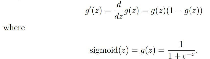
计算sigmoid函数的梯度，公式如下：

sigmoidGradient.m

function g = sigmoidGradient(z)

%SIGMOIDGRADIENT returns the gradient of the sigmoid function

%evaluated at z

%   g = SIGMOIDGRADIENT(z) computes the gradient of the sigmoid function

%   evaluated at z. This should work regardless if z is a matrix or a

%   vector. In particular, if z is a vector or matrix, you should return

%   the gradient for each element.

　　

g = sigmoid(z).*(-sigmoid(z));　　//要求对向量和矩阵同样适用，所以使用点乘而不是直接相乘

end

ex4.m中的调用

%% ================ Part : Sigmoid Gradient  ================

g = sigmoidGradient([ -0.5  0.5 ]);

fprintf('Sigmoid gradient evaluated at [1 -0.5 0 0.5 1]:\n  ');

fprintf('%f ', g);

2.2 随机初始化

在训练神经网络时，随机初始化参数来进行对称破坏非常重要。随机初始化的一个有效策略是在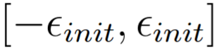

的范围内统一随机选择 θ^（l）的值，你应该使用 ε_init = 0.12。这里对值的选择有一个说明：

randInitializeWeights.m

function W = randInitializeWeights(L_in, L_out)

%RANDINITIALIZEWEIGHTS Randomly initialize the weights of a layer with L_in

%incoming connections and L_out outgoing connections

%   W = RANDINITIALIZEWEIGHTS(L_in, L_out) randomly initializes the weights

%   of a layer with L_in incoming connections and L_out outgoing

%   connections.

%

%   Note that W should be set to a matrix of size(L_out,  + L_in) as

%   the column row of W handles the "bias" terms

epsilon_init = 0.12;

W = rand(L_out,  + L_in) *  * epsilon_init - epsilon_init; 

end

ex4.m 里的调用为：

%% ================ Part : Initializing Pameters ================

initial_Theta1 = randInitializeWeights(input_layer_size, hidden_layer_size);

initial_Theta2 = randInitializeWeights(hidden_layer_size, num_labels);

% Unroll parameters

initial_nn_params = [initial_Theta1(:) ; initial_Theta2(:)];

2.3 反向传播

反向传播算法，由右到左计算误差项 δ_j^(l)：

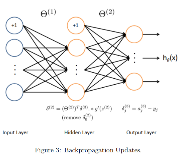
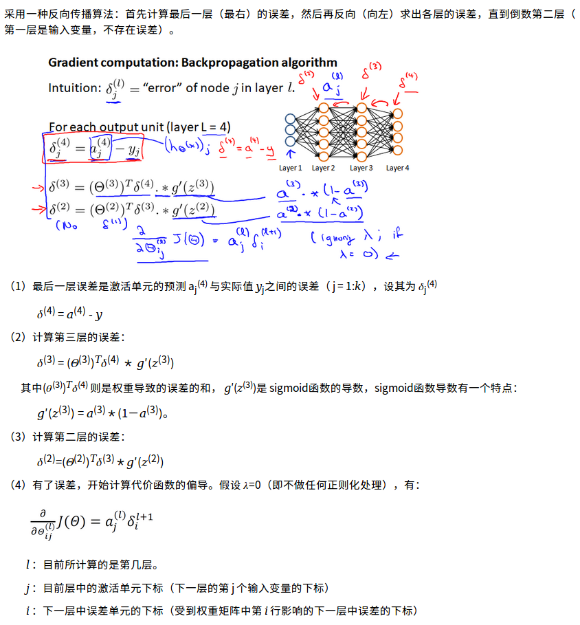
详细请看我的课程笔记：Coursera—Andrew Ng机器学习—课程笔记 Lecture 9_Neural Networks learning

（1）根据上面的公式计算 “误差项 error term”。代码如下：

%----------------------------PART ----------------------------------

% Accumulate the error term

delta_3 = hx - yt;                                               %  x

delta_2 = delta_3 * Theta2 .* sigmoidGradient([ones(m, ) z2]);  %  x  =  x  *  x  .*  x 26

% 去掉 δ₂^（0）这一项

delta_2 = delta_2(:,:end);   　　　　　　　　　　　　　　　　　　　　　　%  x 25

（2）计算梯度，公式和代码如下：

% Accumulate the gradient

D2 = delta_3' * a2;    % 10 x 26 = 10 x 5000 * 5000 x 26

D1 = delta_2' * a1;    % 25 x 401 = 25 x 5000 * 5000 x 401

（4）获得代价函数 J（θ）针对Theta1 和 Theta2 的偏导数，公式和代码如下：

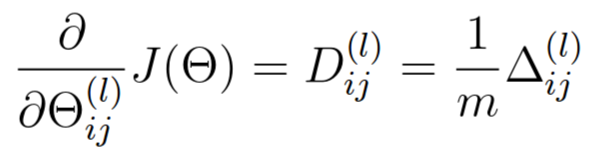
% Obtain the (unregularized) gradient for the neural network cost function

Theta2_grad = /m * D2;

Theta1_grad = /m * D1;

2.4 梯度校验

梯度校验的原理：

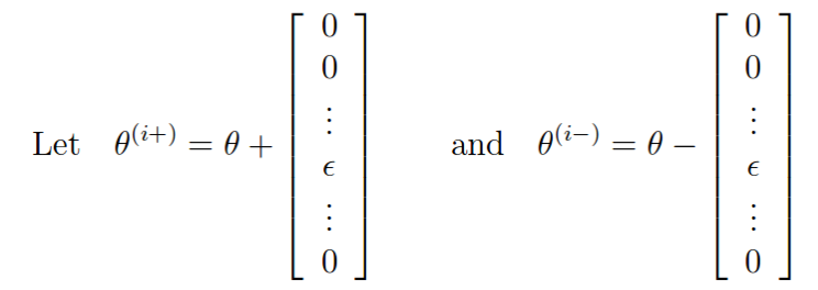
如果梯度计算正确，则下面两个值的差应该比较小

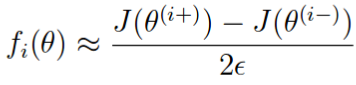
在 computeNumericalGradient.m 中，已经实现了梯度校验的过程，它会生成一个小型神经网络和数据集来进行校验。如果梯度计算正确，会得到一个小于 e^-9的差值。

在真正开始模型学习时，需要关闭梯度校验。

2.5 正则化神经网络

上面计算出的偏导数没有加入正则项，加入正则项的公式如下（ j = 0 不参与正则化，即将θ的第一列置为0）

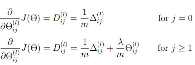
%----------------------------PART ----------------------------------

%---Regularize gradients

temp1 = Theta1;

temp2 = Theta2;

temp1(:,) = ; 　　% set first column to

temp2(:,) = ; 　　% set first column to

Theta1_grad = Theta1_grad + lambda/m * temp1;

Theta2_grad = Theta2_grad + lambda/m * temp2;

ex4.m 中的调用：

%% =============== Part : Implement Regularization ===============

%  Check gradients by running checkNNGradients

lambda = ;

checkNNGradients(lambda);

% Also output the costFunction debugging values

debug_J  = nnCostFunction(nn_params, input_layer_size, ...

                          hidden_layer_size, num_labels, X, y, lambda);

2.6 使用 fmincg 函数训练参数

ex4.m 中的调用如下：

%% =================== Part : Training NN ===================

options = optimset('MaxIter', );

%  You should also try different values of lambda

lambda = ;

% Create "short hand" for the cost function to be minimized

costFunction = @(p) nnCostFunction(p, ...

                                   input_layer_size, ...

                                   hidden_layer_size, ...

                                   num_labels, X, y, lambda);

% Now, costFunction is a function that takes in only one argument (the

% neural network parameters)

[nn_params, cost] = fmincg(costFunction, initial_nn_params, options);% Obtain Theta1 and Theta2 back from nn_params

Theta1 = reshape(nn_params(:hidden_layer_size * (input_layer_size + )), ...

                 hidden_layer_size, (input_layer_size + ));

Theta2 = reshape(nn_params(( + (hidden_layer_size * (input_layer_size + ))):end), ...

                 num_labels, (hidden_layer_size + ));

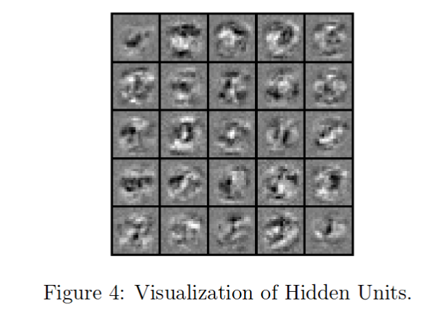
3 可视化hidden layer

如果我们将 Theta1 中的一行拿出来，去掉了第一个 bias term，得到一个 400 维的向量。可视化hidden单元的一种方法，就是将这个 400 维向量重新整形为 20×20 图像，并显示它。

ex4.m 中的调用如下：

%% ================= Part : Visualize Weights =================

displayData(Theta1(:, :end));   % 去掉第一列

图像如下，Theta1 的每一行对应一个小格子：

4 预测

预测准确率为 94.34%。我们引入正则化的作用是避免过拟合，如果将2.6中的 λ 设置为 0 或一个小数值，或者通过调整MaxIter，甚至可能得到一个准确率为100%的模型。但这种模型对于预测新来的数据，表现可能很差。

ex4.m 中的调用如下

%% ================= Part : Implement Predict =================

pred = predict(Theta1, Theta2, X);

5 运行结果

运行ex4.m 得到的结果如下：

Loading and Visualizing Data ...

Program paused. Press enter to continue.

Loading Saved Neural Network Parameters ...

Feedforward Using Neural Network ...

Cost at parameters (loaded from ex4weights): 0.287629

(this value should be about 0.287629)

Program paused. Press enter to continue.

Checking Cost Function (w/ Regularization) ...

Cost at parameters (loaded from ex4weights): 0.383770

(this value should be about 0.383770)

Program paused. Press enter to continue.

Evaluating sigmoid gradient...

Sigmoid gradient evaluated at [ -0.5  0.5 ]:

  0.196612 0.235004 0.250000 0.235004 0.196612 

Program paused. Press enter to continue.

Initializing Neural Network Parameters ...

Checking Backpropagation...

   -0.0093   -0.0093

    0.0089    0.0089

   -0.0084   -0.0084

    0.0076    0.0076

   -0.0067   -0.0067

   -0.0000   -0.0000

    0.0000    0.0000

   -0.0000   -0.0000

    0.0000    0.0000

   -0.0000   -0.0000

   -0.0002   -0.0002

    0.0002    0.0002

   -0.0003   -0.0003

    0.0003    0.0003

   -0.0004   -0.0004

   -0.0001   -0.0001

    0.0001    0.0001

   -0.0001   -0.0001

    0.0002    0.0002

   -0.0002   -0.0002

    0.3145    0.3145

    0.1111    0.1111

    0.0974    0.0974

    0.1641    0.1641

    0.0576    0.0576

    0.0505    0.0505

    0.1646    0.1646

    0.0578    0.0578

    0.0508    0.0508

    0.1583    0.1583

    0.0559    0.0559

    0.0492    0.0492

    0.1511    0.1511

    0.0537    0.0537

    0.0471    0.0471

    0.1496    0.1496

    0.0532    0.0532

    0.0466    0.0466

The above two columns you get should be very similar.

(Left-Your Numerical Gradient, Right-Analytical Gradient)

If your backpropagation implementation is correct, then

the relative difference will be small (less than 1e-). 

Relative Difference: 2.2366e-11

Program paused. Press enter to continue.

Checking Backpropagation (w/ Regularization) ...

   -0.0093   -0.0093

    0.0089    0.0089

   -0.0084   -0.0084

    0.0076    0.0076

   -0.0067   -0.0067

   -0.0168   -0.0168

    0.0394    0.0394

    0.0593    0.0593

    0.0248    0.0248

   -0.0327   -0.0327

   -0.0602   -0.0602

   -0.0320   -0.0320

    0.0249    0.0249

    0.0598    0.0598

    0.0386    0.0386

   -0.0174   -0.0174

   -0.0576   -0.0576

   -0.0452   -0.0452

    0.0091    0.0091

    0.0546    0.0546

    0.3145    0.3145

    0.1111    0.1111

    0.0974    0.0974

    0.1187    0.1187

    0.0000    0.0000

    0.0337    0.0337

    0.2040    0.2040

    0.1171    0.1171

    0.0755    0.0755

    0.1257    0.1257

   -0.0041   -0.0041

    0.0170    0.0170

    0.1763    0.1763

    0.1131    0.1131

    0.0862    0.0862

    0.1323    0.1323

   -0.0045   -0.0045

    0.0015    0.0015

The above two columns you get should be very similar.

(Left-Your Numerical Gradient, Right-Analytical Gradient)

If your backpropagation implementation is correct, then

the relative difference will be small (less than 1e-). 

Relative Difference: 2.17629e-11

Cost at (fixed) debugging parameters (w/ lambda = ): 0.576051

(this value should be about 0.576051)

Program paused. Press enter to continue.

Training Neural Network...

Iteration      | Cost: 3.298708e+00

Iteration      | Cost: 3.254768e+00

Iteration      | Cost: 3.209718e+00

Iteration      | Cost: 3.124366e+00

Iteration      | Cost: 2.858652e+00

Iteration      | Cost: 2.454280e+00

Iteration      | Cost: 2.259612e+00

Iteration      | Cost: 2.184967e+00

Iteration      | Cost: 1.895567e+00

Iteration     | Cost: 1.794052e+00

Iteration     | Cost: 1.658111e+00

Iteration     | Cost: 1.551086e+00

Iteration     | Cost: 1.440756e+00

Iteration     | Cost: 1.319321e+00

Iteration     | Cost: 1.218193e+00

Iteration     | Cost: 1.174144e+00

>>

Iteration     | Cost: 1.121406e+00

Iteration     | Cost: 1.001795e+00

Iteration     | Cost: 9.730070e-01

Iteration     | Cost: 9.396211e-01

Iteration     | Cost: 8.982489e-01

Iteration     | Cost: 8.785754e-01

Iteration     | Cost: 8.558708e-01

Iteration     | Cost: 8.358078e-01

Iteration     | Cost: 8.074475e-01

Iteration     | Cost: 7.975287e-01

Iteration     | Cost: 7.883648e-01

Iteration     | Cost: 7.543000e-01

Iteration     | Cost: 7.318456e-01

Iteration     | Cost: 7.151468e-01

Iteration     | Cost: 6.919630e-01

Iteration     | Cost: 6.823971e-01

Iteration     | Cost: 6.766813e-01

Iteration     | Cost: 6.639429e-01

Iteration     | Cost: 6.579100e-01

Iteration     | Cost: 6.491120e-01

Iteration     | Cost: 6.405250e-01

Iteration     | Cost: 6.318625e-01

Iteration     | Cost: 6.180036e-01

Iteration     | Cost: 6.081649e-01

Iteration     | Cost: 5.973954e-01

Iteration     | Cost: 5.684440e-01

Iteration     | Cost: 5.465935e-01

Iteration     | Cost: 5.399081e-01

Iteration     | Cost: 5.320386e-01

Iteration     | Cost: 5.289632e-01

Iteration     | Cost: 5.252995e-01

Iteration     | Cost: 5.236517e-01

Iteration     | Cost: 5.233562e-01

Iteration     | Cost: 5.197894e-01

Program paused. Press enter to continue.

Visualizing Neural Network... 

Program paused. Press enter to continue.

Training Set Accuracy: 94.340000

完整代码

https://github.com/madoubao/coursera_machine_learning/tree/master/homework/machine-learning-ex4/ex4