VBA在Excel中的应用(三)
目录
 Chart Export Chart Format Chart Lengend Chart Protect Chart Title Chart
Chart Export
- 1. 将Excel中的图表导出成gif格式的图片保存到硬盘上
Sub ExportChart()

    Dim myChart As Chart

    Set myChart = ActiveChart

    myChart.Export Filename:="C:\Chart.gif", Filtername:="GIF"

End Sub
理论上图表可以被保存成任何类型的图片文件,读者可以自己去尝试。
- 2. 将Excel中的图表导出成可交互的页面保存到硬盘上
Sub SaveChartWeb()

    ActiveWorkbook.PublishObjects.Add _

        SourceType:=xlSourceChart, _

        Filename:=ActiveWorkbook.Path & "\Sample2.htm", _

        Sheet:=ActiveSheet.name, _

        Source:=" Chart 1", _

        HtmlType:=xlHtmlChart

    ActiveWorkbook.PublishObjects(1).Publish (True)

End Sub
Chart Format
- 1. 操作Chart对象。给几个用VBA操作Excel Chart对象的例子,读者可以自己去尝试一下。
Public Sub ChartInterior()

    Dim myChart As Chart

    'Reference embedded chart

    Set myChart = ActiveSheet.ChartObjects(1).Chart

    With myChart   'Alter interior colors of chart components

        .ChartArea.Interior.Color = RGB(1, 2, 3)

        .PlotArea.Interior.Color = RGB(11, 12, 1)

        .Legend.Interior.Color = RGB(31, 32, 33)

        If .HasTitle Then

            .ChartTitle.Interior.Color = RGB(41, 42, 43)

        End If

    End With

End Sub
Public Sub SetXAxis()
Dim myAxis As Axis
Set myAxis = ActiveSheet.ChartObjects(1).Chart.Axes(xlCategory, xlPrimary)
With myAxis 'Set properties of x-axis
.HasMajorGridlines = True
.HasTitle = True
.AxisTitle.Text = "My Axis"
.AxisTitle.Font.Color = RGB(1, 2, 3)
.CategoryNames = Range("C2:C11")
.TickLabels.Font.Color = RGB(11, 12, 13)
End With
End SubPublic Sub TestSeries()
Dim mySeries As Series
Dim seriesCol As SeriesCollection
Dim I As Integer
I = 1
Set seriesCol = ActiveSheet.ChartObjects(1).Chart.SeriesCollection
For Each mySeries In seriesCol
Set mySeries = ActiveSheet.ChartObjects(1).Chart.SeriesCollection(I)
With mySeries
.MarkerBackgroundColor = RGB(1, 32, 43)
.MarkerForegroundColor = RGB(11, 32, 43)
.Border.Color = RGB(11, 12, 23)
End With
I = I + 1
Next
End SubPublic Sub TestPoint()
Dim myPoint As Point
Set myPoint = ActiveSheet.ChartObjects(1).Chart.SeriesCollection(1).Points(3)
With myPoint
.ApplyDataLabels xlDataLabelsShowValue
.MarkerBackgroundColor = RGB(1, 2, 3)
.MarkerForegroundColor = RGB(11, 22, 33)
End With
End SubSub chartAxis()
Dim myChartObject As ChartObject
Set myChartObject = ActiveSheet.ChartObjects.Add(Left:=200, Top:=200, _
Width:=400, Height:=300)
myChartObject.Chart.SetSourceData Source:= _
ActiveWorkbook.Sheets("Chart Data").Range("A1:E5")
myChartObject.SeriesCollection.Add Source:=ActiveSheet.Range("C4:K4"), Rowcol:=xlRows
myChartObject.SeriesCollection.NewSeries
myChartObject.HasTitle = True
With myChartObject.Axes(Type:=xlCategory, AxisGroup:=xlPrimary)
.HasTitle = True
.AxisTitle.Text = "Years"
.AxisTitle.Font.Name = "Times New Roman"
.AxisTitle.Font.Size = 12
.HasMajorGridlines = True
.HasMinorGridlines = False
End With
End SubSub FormattingCharts()
Dim myChart As Chart
Dim ws As Worksheet
Dim ax As Axis Set ws = ThisWorkbook.Worksheets("Sheet1")
Set myChart = GetChartByCaption(ws, "GDP") If Not myChart Is Nothing Then
Set ax = myChart.Axes(xlCategory)
With ax
.AxisTitle.Font.Size = 12
.AxisTitle.Font.Color = vbRed
End With
Set ax = myChart.Axes(xlValue)
With ax
.HasMinorGridlines = True
.MinorGridlines.Border.LineStyle = xlDashDot
End With
With myChart.PlotArea
.Border.LineStyle = xlDash
.Border.Color = vbRed
.Interior.Color = vbWhite
.Width = myChart.PlotArea.Width + 10
.Height = myChart.PlotArea.Height + 10
End With
myChart.ChartArea.Interior.Color = vbWhite
myChart.Legend.Position = xlLegendPositionBottom
End If Set ax = Nothing
Set myChart = Nothing
Set ws = Nothing
End Sub
Function GetChartByCaption(ws As Worksheet, sCaption As String) As Chart
Dim myChart As ChartObject
Dim myChart As Chart
Dim sTitle As String Set myChart = Nothing
For Each myChart In ws.ChartObjects
If myChart.Chart.HasTitle Then
sTitle = myChart.Chart.ChartTitle.Caption
If StrComp(sTitle, sCaption, vbTextCompare) = 0 Then
Set myChart = myChart.Chart
Exit For
End If
End If
Next
Set GetChartByCaption = myChart
Set myChart = Nothing
Set myChart = Nothing
End Function - 2. 使用VBA在Excel中添加图表
Public Sub AddChartSheet()

  Dim aChart As Chart

  Set aChart = Charts.Add

  With aChart

    .Name = "Mangoes"

    .ChartType = xlColumnClustered

    .SetSourceData Source:=Sheets("Sheet1").Range("A3:D7"), PlotBy:=xlRows

    .HasTitle = True

    .ChartTitle.Text = "=Sheet1!R3C1"

  End With

End Sub - 3. 遍历并更改Chart对象中的图表类型
Sub ChartType()

    Dim myChart As ChartObject

    For Each myChart In ActiveSheet.ChartObjects

        myChart.Chart.Type = xlArea

    Next myChart

End Sub - 4. 遍历并更改Chart对象中的Legend
Sub LegendMod()

    Dim myChart As ChartObject

    For Each myChart In ActiveSheet.ChartObjects

        With myChart.Chart.Legend.font

            .name = "Calibri"

            .FontStyle = "Bold"

            .Size = 12

        End With

    Next myChart

End Sub - 5. 一个格式化Chart的例子
Sub ChartMods()

    ActiveChart.Type = xlArea

    ActiveChart.ChartArea.font.name = "Calibri"

    ActiveChart.ChartArea.font.FontStyle = "Regular"

    ActiveChart.ChartArea.font.Size = 9

    ActiveChart.PlotArea.Interior.ColorIndex = xlNone

    ActiveChart.Axes(xlValue).TickLabels.font.bold = True

    ActiveChart.Axes(xlCategory).TickLabels.font.bold = True

    ActiveChart.Legend.Position = xlBottom

End Sub - 6. 通过VBA更改Chart的Title
Sub ApplyTexture()

    Dim myChart As Chart

    Dim ser As Series

    Set myChart = ActiveChart

    Set ser = myChart.SeriesCollection(2)

    ser.Format.Fill.PresetTextured (msoTextureGreenMarble)

End Sub - 7. 在VBA中使用自定义图片填充Chart对象的series区域
Sub FormatWithPicture()

    Dim myChart As Chart

    Dim ser As Series

    Set myChart = ActiveChart

    Set ser = myChart.SeriesCollection(1)

    MyPic = "C:\Title.jpg"

    ser.Format.Fill.UserPicture (MyPic)

End Sub
Excel中的Chart允许用户对其中选定的区域自定义样式,其中包括使用图片选中样式。在Excel的Layout菜单下有一个Format Selection,首先在Chart对象中选定要格式化的区域,例如series,然后选择该菜单,在弹出的对话框中即可对所选的区域进行格式化。如series选项、填充样式、边框颜色和样式、阴影以及3D效果等。下面再给出一个在VBA中使用渐变色填充Chart对象的series区域的例子。
Sub TwoColorGradient()

    Dim myChart As Chart

    Dim ser As Series

    Set myChart = ActiveChart

    Set ser = myChart.SeriesCollection(1)

    MyPic = "C:\Title1.jpg"

    ser.Format.Fill.TwoColorGradient msoGradientFromCorner, 3

    ser.Format.Fill.ForeColor.ObjectThemeColor = msoThemeColorAccent6

    ser.Format.Fill.BackColor.ObjectThemeColor = msoThemeColorAccent2

End Sub - 8. 通过VBA格式化Chart对象中series的趋势线样式
Sub FormatLineOrBorders()

    Dim myChart As Chart

    Set myChart = ActiveChart

    With myChart.SeriesCollection(1).Trendlines(1).Format.Line

        .DashStyle = msoLineLongDashDotDot

        .ForeColor.RGB = RGB(50, 0, 128)

        .BeginArrowheadLength = msoArrowheadShort

        .BeginArrowheadStyle = msoArrowheadOval

        .BeginArrowheadWidth = msoArrowheadNarrow

        .EndArrowheadLength = msoArrowheadLong

        .EndArrowheadStyle = msoArrowheadTriangle

        .EndArrowheadWidth = msoArrowheadWide

    End With

End Sub
Excel允许用户为Chart对象的series添加趋势线(trendline),首先在Chart中选中要设置的series,然后选择Layout菜单下的trendline,选择一种trendline样式。
- 9. 一组利用VBA格式化Chart对象的例子
Sub FormatBorder()

    Dim myChart As Chart

    Set myChart = ActiveChart

    With myChart.ChartArea.Format.Line

        .DashStyle = msoLineLongDashDotDot

        .ForeColor.RGB = RGB(50, 0, 128)

    End With

End Sub
Sub AddGlowToTitle()
Dim myChart As Chart
Set myChart = ActiveChart
myChart.ChartTitle.Format.Line.ForeColor.RGB = RGB(255, 255, 255)
myChart.ChartTitle.Format.Line.DashStyle = msoLineSolid
myChart.ChartTitle.Format.Glow.Color.ObjectThemeColor = msoThemeColorAccent6
myChart.ChartTitle.Format.Glow.Radius = 8
End SubSub FormatShadow()
Dim myChart As Chart
Set myChart = ActiveChart
With myChart.Legend.Format.Shadow
.ForeColor.RGB = RGB(0, 0, 128)
.OffsetX = 5
.OffsetY = -3
.Transparency = 0.5
.Visible = True
End With
End SubSub FormatSoftEdgesWithLoop()
Dim myChart As Chart
Dim ser As Series
Set myChart = ActiveChart
Set ser = myChart.SeriesCollection(1)
For i = 1 To 6
ser.Points(i).Format.SoftEdge.Type = i
Next i
End Sub - 10. 在VBA中对Chart对象应用3D效果
Sub Assign3DPreset()

    Dim myChart As Chart

    Dim shp As Shape

    Set myChart = ActiveChart

    Set shp = myChart.Shapes(1)

    shp.ThreeD.SetPresetCamera msoCameraIsometricLeftDown

End Sub
Sub AssignBevel()
Dim myChart As Chart
Dim ser As Series
Set myChart = ActiveChart
Set ser = myChart.SeriesCollection(1)
ser.Format.ThreeD.Visible = True
ser.Format.ThreeD.BevelTopType = msoBevelCircle
ser.Format.ThreeD.BevelTopInset = 16
ser.Format.ThreeD.BevelTopDepth = 6
End Sub
Chart Lengend
- 1. 设置Lengend的位置和ChartArea的颜色
Sub FormattingCharts()

    Dim myChart As Chart

    Dim ws As Worksheet

    Dim ax As Axis

    Set ws = ThisWorkbook.Worksheets("Sheet1")

    Set myChart = GetChartByCaption(ws, "GDP")

    If Not myChart Is Nothing Then

        myChart.ChartArea.Interior.Color = vbWhite

        myChart.Legend.Position = xlLegendPositionBottom

    End If

    Set ax = Nothing

    Set myChart = Nothing

    Set ws = Nothing

End Sub

Function GetChartByCaption(ws As Worksheet, sCaption As String) As Chart

    Dim myChart As ChartObject

    Dim myChart As Chart

    Dim sTitle As String

    Set myChart = Nothing

    For Each myChart In ws.ChartObjects

        If myChart.Chart.HasTitle Then

            sTitle = myChart.Chart.ChartTitle.Caption

            If StrComp(sTitle, sCaption, vbTextCompare) = 0 Then

                Set myChart = myChart.Chart

                Exit For

            End If

        End If

    Next

    Set GetChartByCaption = myChart

    Set myChart = Nothing

    Set myChart = Nothing

End Function - 2. 通过VBA给Chart添加Lengend
Sub legend()

    Dim myChartObject As ChartObject

    Set myChartObject = ActiveSheet.ChartObjects.Add(Left:=200, Top:=200, _

        Width:=400, Height:=300)


    myChartObject.Chart.SetSourceData Source:= _

        ActiveWorkbook.Sheets("Chart Data").Range("A1:E5")


    myChartObject.SeriesCollection.Add Source:=ActiveSheet.Range("C4:K4"), Rowcol:=xlRows

    myChartObject.SeriesCollection.NewSeries

    With myChartObject.Legend

        .HasLegend = True

        .Font.Size = 16

        .Font.Name = "Arial"

    End With

End Sub
Chart Protect
- 1. 保护图表
Sub ProtectChart()

    Dim myChart As Chart

    Set myChart = ThisWorkbook.Sheets("Protected Chart")

    myChart.Protect "123456", True, True, , True

    myChart.ProtectData = False

    myChart.ProtectGoalSeek = True

    myChart.ProtectSelection = True

End Sub
Excel中的Chart可以和Sheet一样被保护,读者可以选中图表所在的Tab,然后通过Review菜单下的Protect Sheet菜单来对图表进行保护设置。代码中的Protected Chart123456是设置保护时的密码,有关Protect函数的参数和设置保护时的其它属性读者可以查阅Excel自带的帮助文档。
- 2. 取消图表保护
Sub UnprotectChart()

    Dim myChart As Chart

    Set myChart = ThisWorkbook.Sheets("Protected Chart")

    myChart.Unprotect "123456"

    myChart.ProtectData = False

    myChart.ProtectGoalSeek = False

    myChart.ProtectSelection = False

End Sub
与保护图表的示例相对应,可以通过VBA撤销对图表的保护设置。
Chart Title
- 1. 通过VBA添加图表的标题
Sub chartTitle()

    Dim myChartObject As ChartObject

    Set myChartObject = ActiveSheet.ChartObjects.Add(Left:=200, Top:=200, _

        Width:=400, Height:=300)


    myChartObject.Chart.SetSourceData Source:= _

        ActiveWorkbook.Sheets("Chart Data").Range("A1:E5")


    myChartObject.SeriesCollection.Add Source:=ActiveSheet.Range("C4:K4"), Rowcol:=xlRows

    myChartObject.SeriesCollection.NewSeries

    myChartObject.HasTitle = True

End Sub
如果要设置标题显示的位置,可以在上述代码的后面加上:
With myChartObject.ChartTitle
.Top =
.Left =
End With
如果要同时设置标题字体,可以在上述代码的后面加上:
myChartObject.ChartTitle.Font.Name = "Times" - 2. 通过VBA修改图表的标题
Sub charTitleText()

    ActiveChart.ChartTitle.Text = "Industrial Disease in North Dakota"

End Sub - 3. 一个通过标题搜索图表的例子
Function GetChartByCaption(ws As Worksheet, sCaption As String) As Chart

    Dim myChart As ChartObject

    Dim myChart As Chart

    Dim sTitle As String

    Set myChart = Nothing

    For Each myChart In ws.ChartObjects

        If myChart.Chart.HasTitle Then

            sTitle = myChart.Chart.ChartTitle.Caption

            If StrComp(sTitle, sCaption, vbTextCompare) = 0 Then

                Set myChart = myChart.Chart

                Exit For

            End If

        End If

    Next

    Set GetChartByCaption = myChart

    Set myChart = Nothing

    Set myChart = Nothing

End Function

Sub TestGetChartByCaption()

    Dim myChart As Chart

    Dim ws As Worksheet

    Set ws = ThisWorkbook.Worksheets("Sheet1")

    Set myChart = GetChartByCaption(ws, "I am the Chart Title")

    If Not myChart Is Nothing Then

        Debug.Print "Found chart"

    Else

        Debug.Print "Sorry - chart not found"

    End If

    Set ws = Nothing

    Set myChart = Nothing

End Sub
Chart
- 1. 通过VBA创建Chart的几种方式
使用ChartWizard方法创建Sub CreateExampleChartVersionI()
Dim ws As Worksheet
Dim rgChartData As Range
Dim myChart As Chart Set ws = ThisWorkbook.Worksheets("Sheet1")
Set rgChartData = ws.Range("B1").CurrentRegion
Set myChart = Charts.Add
Set myChart = myChart.Location(xlLocationAsObject, ws.Name)
With myChart
.ChartWizard _
Source:=rgChartData, _
Gallery:=xlColumn, _
Format:=1, _
PlotBy:=xlColumns, _
CategoryLabels:=1, _
SeriesLabels:=1, _
HasLegend:=True, _
Title:="Version I", _
CategoryTitle:="Year", _
ValueTitle:="GDP in billions of $"
End With Set myChart = Nothing
Set rgChartData = Nothing
Set ws = Nothing
End Sub使用Chart Object方法创建
Sub CreateExampleChartVersionII()

    Dim ws As Worksheet

    Dim rgChartData As Range

    Dim myChart As Chart

    Set ws = ThisWorkbook.Worksheets("Basic Chart")

    Set rgChartData = ws.Range("B1").CurrentRegion

    Set myChart = Charts.Add

    Set myChart = myChart.Location(xlLocationAsObject, ws.Name)

    With myChart

        .SetSourceData rgChartData, xlColumns

        .HasTitle = True

        .ChartTitle.Caption = "Version II"

        .ChartType = xlColumnClustered

        With .Axes(xlCategory)

            .HasTitle = True

            .AxisTitle.Caption = "Year"

        End With

        With .Axes(xlValue)

            .HasTitle = True

            .AxisTitle.Caption = "GDP in billions of $"

        End With

    End With

    Set myChart = Nothing

    Set rgChartData = Nothing

    Set ws = Nothing

End Sub
使用ActiveWorkbook.Sheets.Add方法创建
Sub chart()

    Dim myChartSheet As Chart

    Set myChartSheet = ActiveWorkbook.Sheets.Add _

        (After:=ActiveWorkbook.Sheets(ActiveWorkbook.Sheets.Count), _

        Type:=xlChart)

End Sub
使用ActiveSheet.ChartObjects.Add方法创建
Sub charObj()

    Dim myChartObject As ChartObject

    Set myChartObject = ActiveSheet.ChartObjects.Add(Left:=200, Top:=200, _

        Width:=400, Height:=300)

    myChartObject.Chart.SetSourceData Source:= _

        ActiveWorkbook.Sheets("Chart Data").Range("A1:E5")

End Sub
不同的创建方法可以应用在不同的场合,如Sheet中内嵌的图表,一个独立的Chart Tab等,读者可以自己研究。最后一种方法的末尾给新创建的图表设定了数据源,这样图表就可以显示出具体的图形了。
如果需要指定图表的类型,可以加上这句代码:
myChartObject.ChartType = xlColumnStacked
如果需要在现有图表的基础上添加新的series,下面这行代码可以参考:
myChartObject.SeriesCollection.Add Source:=ActiveSheet.Range("C4:K4"), Rowcol:=xlRows
或者通过下面这行代码对已有的series进行扩展:
myChartObject.SeriesCollection.Extend Source:=Worksheets("Chart Data").Range("P3:P8") - 2. 一个相对完整的通过VBA创建Chart的例子
'Common Excel Chart Types

'-------------------------------------------------------------------

'Chart   |   VBA Constant (ChartType property of Chart object)     |

'==================================================================

'Column  |   xlColumnClustered, xlColumnStacked, xlColumnStacked100|

'Bar     |   xlBarClustered, xlBarStacked, xlBarStacked100         |

'Line    |   xlLine, xlLineMarkersStacked, xlLineStacked           |

'Pie     |   xlPie, xlPieOfPie                                     |

'Scatter |   xlXYScatter, xlXYScatterLines                         |

'-------------------------------------------------------------------

Public Sub AddChartSheet()

    Dim dataRange As Range

    Set dataRange = ActiveWindow.Selection

    Charts.Add   'Create a chart sheet

    With ActiveChart    'Set chart properties

        .ChartType = xlColumnClustered

        .HasLegend = True

        .Legend.Position = xlRight

        .Axes(xlCategory).MinorTickMark = xlOutside

        .Axes(xlValue).MinorTickMark = xlOutside

        .Axes(xlValue).MaximumScale = _

                    Application.WorksheetFunction.RoundUp( _

                    Application.WorksheetFunction.Max(dataRange), -1)

        .Axes(xlCategory).HasTitle = True

        .Axes(xlCategory).AxisTitle.Characters.Text = "X-axis Labels"

        .Axes(xlValue).HasTitle = True

        .Axes(xlValue).AxisTitle.Characters.Text = "Y-axis"

        .SeriesCollection(1).name = "Sample Data"

        .SeriesCollection(1).Values = dataRange

    End With

End Sub - 3. 通过选取的Cells Range的值设置Chart中数据标签的内容
Sub DataLabelsFromRange()

    Dim DLRange As range

    Dim myChart As Chart

    Dim i As Integer


    Set myChart = ActiveSheet.ChartObjects(1).Chart

    On Error Resume Next

    Set DLRange = Application.InputBox _

      (prompt:="Range for data labels?", Type:=8)

    If DLRange Is Nothing Then Exit Sub

    On Error GoTo 0

    myChart.SeriesCollection(1).ApplyDataLabels Type:=xlDataLabelsShowValue, AutoText:=True, LegendKey:=False

    Pts = myChart.SeriesCollection(1).Points.Count

    For i = 1 To Pts

        myChart.SeriesCollection(1). _

          Points(i).DataLabel.Characters.Text = DLRange(i)

    Next i

End Sub
考虑下面这个场景,当采用下表的数据生成图表Chart4时,默认的效果如下图。
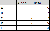
 可以手动给该图表添加Data Labels,方法是选中任意的series,右键选择Add Data Labels。如果想要为所有的series添加Data Labels,则需要依次选择不同的series,然后重复该操作。
Excel中可以通过VBA将指定Cells Range中的值设置到Chart的Data Labels中,上面的代码就是一个例子。程序执行的时候会首先弹出一个提示框,要求用户通过鼠标去选择一个单元格区域以获取到Cells集合(或者直接输入地址),如下图: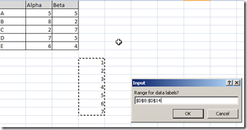 注意VBA中输入型对话框Application.InputBox的使用。在循环中将Range中的值添加到Chart的Data Labels中。
 - 4. 一个使用VBA给Chart添加Data Labels的例子
Sub AddDataLabels()

    Dim seSales As Series

    Dim pts As Points

    Dim pt As Point

    Dim rngLabels As range

    Dim iPointIndex As Integer

    Set rngLabels = range("B4:G4")

    Set seSales = ActiveSheet.ChartObjects(1).Chart.SeriesCollection(1)

    seSales.HasDataLabels = True

    Set pts = seSales.Points

    For Each pt In pts

        iPointIndex = iPointIndex + 1

        pt.DataLabel.text = rngLabels.cells(iPointIndex).text

        pt.DataLabel.font.bold = True

        pt.DataLabel.Position = xlLabelPositionAbove

    Next pt

End Sub
VBA在Excel中的应用(三)的更多相关文章
- VBA在Excel中的应用(一):改变符合条件单元格的背景颜色
在使用excel处理数据的时候,为了能更清晰的标示出满足特定条件的单元格,对单元格添加背景色是不错的选择.手工处理的方式简单快捷,但是当遇到大批量数据,就会特别的费时费力,而且不讨好(容易出错).通过 ...
- 利用VBA查找excel中一行某列第一次不为空与最后一列不为空的列数
昨日同事有需求,想知道每个商品第一次销售的月份,以及最后一次销售的月份. 本想通过什么excel函数来解决,但是找了半天也没找到合适的,最后还是通过VBA来解决吧. 使用方法: Excel工具-宏-V ...
- excel中vba将excel中数字和图表输出到word中
参考:https://wenku.baidu.com/view/6c60420ecc175527072208af.html 比如将选区变为图片保存到桌面: Sub 将选区转为图片存到桌面() Dim ...
- VBA在EXCEL中创建图形线条
EXCEL使用了多少行: ActiveSheet.UsedRange.Rows.Count(再也不用循环到头啦) 创建线条并命名:ActiveSheet.Shapes.AddLine(x1,y1,x2 ...
- 利用vba将excel中的图片链接直接转换为图片
Sub test() Dim rg As Range, shp As Shape Rem --------------------------------------------------- Rem ...
- VBA 删除Excel中所有的图片
Sub DeletePic() Dim p As Shape For Each p In Sheet1.Shapes If p.Type = Then ...
- 如何在open xml excel 中存储自定义xml数据?
如何在open xml excel 中存储自定义xml数据? 而且不能放在隐藏的cell单元格内,也不能放在隐藏的sheet内,要类似web网站的Application变量,但还不能是VBA和宏之类的 ...
- Excel中的宏--VBA的简单例子
第一步:点击录制宏 第二步:填写宏的方法名 第三步:进行一系列的操作之后,关闭宏 第四步:根据自己的需要查看,修改宏 第六步:保存,一般是另存为,后缀名为.xlsm,否则宏语言不能保存. 到此为止恭喜 ...
- Excel中使用VBA访问Access数据库
VBA访问Access数据库 1. 通用自动化语言VBA VBA(Visual Basic For Application)是一种通用自动化语言,它可以使Excel中的常用操作自动化,还可以创建自定义 ...
随机推荐
- 【ABAP系列】SAP ABAP诠释BDC的OK CODE含义
公众号:SAP Technical 本文作者:matinal 原文出处:http://www.cnblogs.com/SAPmatinal/ 原文链接:[ABAP系列]SAP ABAP诠释BDC的OK ...
- WPF资源字典的使用
1.在解决方案中添加资源字典:鼠标右键——添加——资源字典 2.在资源字典中写入你需要的样式,我这里简单的写了一个窗体的边框样式 3.在App.xaml中加入刚刚新建的资源字典就好了
- Node.js实战10:“流”是Node.js最强大的功能之一。
流是Nodejs的高级应用,掌握流的使用,才能真正胜任NodeJS开发. Nodejs中,流是基于事件的API,用于管理和处理数据,而且效率很好! 什么是流? 流是一个抽象接口,Node 中有很多对象 ...
- PyTorch笔记之 scatter() 函数
scatter() 和 scatter_() 的作用是一样的,只不过 scatter() 不会直接修改原来的 Tensor,而 scatter_() 会 PyTorch 中,一般函数加下划线代表直接在 ...
- type动态创建类
在一些特定场合,需要动态创建类,比如创建表单,就会用到type动态创建类,举个例子: class Person(object): def __init__(self,name,age): self.n ...
- 实列+JVM讲解类的实列化顺序
刨根问底---类的实列化顺序 开篇三问 1什么是类的加载,类的加载和类的实列有什么关系,什么时候类加载 2类加载会调用构造函数吗,什么时候调用构造函数 3什么是实列化对象,实列化的对象有什么东西. 我 ...
- 厉害了,Apache架构师们遵循的 30 条设计原则
作者:Srinath 翻译:贺卓凡,来源:公众号ImportSource Srinath通过不懈的努力最终总结出了30条架构原则,他主张架构师的角色应该由开发团队本身去扮演,而不是专门有个架构师团队或 ...
- Codeforces Round #545 (Div. 2) C. Skyscrapers (离散化)
题目传送门 题意: 给你n*m个点,每个点有高度h [ i ][ j ] ,用[1,x][1,x]的数对该元素所处十字上的所有元素重新标号, 并保持它们的相对大小不变.n,m≤1000n,m≤1000 ...
- web框架的本质(使用socket实现的最基础的web框架、使用wsgiref实现的web框架)
import socket def handle_request(client): data = client.recv(1024) client.send("HTTP/1.1 200 OK ...
- 输入某人出生日期(以字符串方式输入,如1987-4-1)使用DateTime和TimeSpan类,(1)计算其人的年龄;(2)计算从现在到其60周岁期间,总共多少天。
http://blog.csdn.net/w92a01n19g/article/details/8764116 using System;using System.Collections.Generi ...