sklearn.metrics中的评估方法

https://www.cnblogs.com/mindy-snail/p/12445973.html

1.confusion_matrix

• 利用混淆矩阵进行评估

• 混淆矩阵说白了就是一张表格-

• 所有正确的预测结果都在对角线上，所以从混淆矩阵中可以很方便直观的看出哪里有错误，因为他们呈现在对角线外面。
  

• 举个直观的例子
  
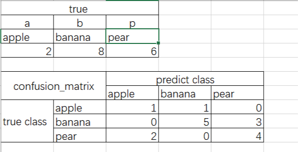
  这个表格是一个混淆矩阵

正确的值是上边的表格，混淆矩阵是下面的表格，这就表示，apple应该有两个，但是只预测对了一个，其中一个判断为banana了，banana应该有8ge，但是5个预测对了3个判断为pear了，pear有应该有6个，但是2个判断为apple了，可见对角线上是正确的预测值，对角线之外的都是错误的。
这个混淆矩阵的实现代码

from sklearn.metrics import confusion_matrix
from sklearn.metrics import classification_report
y_test=["a","b","p","b","b","b","b","p","b","p","b","b","p","p","p","a"]
y_pred=["a","b","p","p","p","p","b","p","b","p","b","b","a","a","p","b"]
confusion_matrix(y_test, y_pred,labels=["a", "b","p"])
#array([[1, 1, 0],
       [0, 5, 3],
       [2, 0, 4]], dtype=int64)

print(classification_report(y_test,y_pred))
##
               precision    recall  f1-score   support

          a       0.33      0.50      0.40         2
          b       0.83      0.62      0.71         8
          p       0.57      0.67      0.62         6

avg / total       0.67      0.62      0.64        16

我传到github上面了

复现代码1

# Import necessary modules
from sklearn.metrics import classification_report

from sklearn.metrics import confusion_matrix

# Create training and test set
X_train, X_test, y_train, y_test = train_test_split(X,y,test_size=0.4,random_state=42)

# Instantiate a k-NN classifier: knn
knn = KNeighborsClassifier(6)

# Fit the classifier to the training data
knn.fit(X_train,y_train)

# Predict the labels of the test data: y_pred
y_pred = knn.predict(X_test)

# Generate the confusion matrix and classification report
print(confusion_matrix(y_test,y_pred))
print(classification_report(y_test,y_pred))

复现代码2

补充知识

先给一个二分类的例子
其他同理

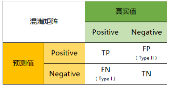
• TP(True Positive)：将正类预测为正类数，真实为0，预测也为0
• FN(False Negative)：将正类预测为负类数，真实为0，预测为1
• FP(False Positive)：将负类预测为正类数， 真实为1，预测为0
• TN(True Negative)：将负类预测为负类数，真实为1，预测也为1

因此:预测性分类模型，肯定是希望越准越好。那么，对应到混淆矩阵中，那肯定是希望TP与TN的数量大，而FP与FN的数量小。所以当我们得到了模型的混淆矩阵后，就需要去看有多少观测值在第二、四象限对应的位置，这里的数值越多越好；反之，在第一、三四象限对应位置出现的观测值肯定是越少越好。

几个二级指标定义

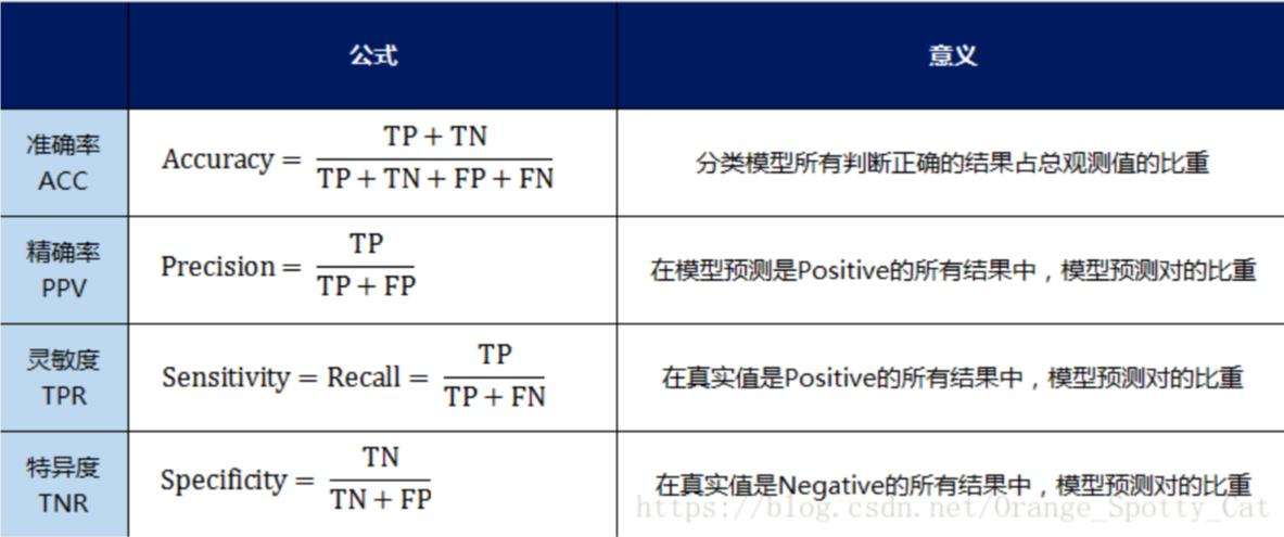
• 准确率（Accuracy）—— 针对整个模型
  \(\frac{t p+t n}{t p+t n+f p+f n}\)
• 精确率（Precision）
  \(\frac{t p}{t p+f n}\)
• 灵敏度（Sensitivity）：就是召回率（Recall）召回率 = 提取出的正确信息条数 / 样本中的信息条数。通俗地说，就是所有准确的条目有多少被检索出来了
• 特异度（Specificity）
  

三级指标

\(\mathrm{F} 1\) Score \(=\frac{2 \mathrm{PR}}{\mathrm{P}+\mathrm{R}}\)
其中，P代表Precision，R代表Recall。
F1-Score指标综合了Precision与Recall的产出的结果。F1-Score的取值范围从0到1的，1代表模型的输出最好，0代表模型的输出结果最差reference

2.accuracy_score()

分类准确率分数

• 分类准确率分数是指所有分类正确的百分比。分类准确率这一衡量分类器的标准比较容易理解，但是它不能告诉你响应值的潜在分布，并且它也不能告诉你分类器犯错的类型

sklearn.metrics.accuracy_score(y_true, y_pred, normalize=True, sample_weight=None)
#normalize：默认值为True，返回正确分类的比例；如果为False，返回正确分类的样本数

复现代码1

#accuracy_score
import numpy as np
from sklearn.metrics import accuracy_score
y_pred = [1, 9, 9, 5,1,0,2,2]
y_true = [1,9,9,8,0,6,1,2]
print(accuracy_score(y_true, y_pred))
print(accuracy_score(y_true, y_pred, normalize=False))
# 0.5
# 4

复现代码2

datacamp上面的一个例子

# Import necessary modules
from sklearn.neighbors import KNeighborsClassifier
from sklearn.model_selection import train_test_split

# Create feature and target arrays
X = digits.data
y = digits.target

# Split into training and test set
X_train, X_test, y_train, y_test = train_test_split(X, y, test_size = 0.2, random_state=42, stratify=y)

# Create a k-NN classifier with 7 neighbors: knn
knn = KNeighborsClassifier(n_neighbors=7)

# Fit the classifier to the training data
knn.fit(X_train, y_train)
y_pred=knn.predict(X_test)
# Print the accuracy
print(accuracy_score(y_test, y_pred))

#0.89996709

ROC

• ROC曲线指受试者工作特征曲线/接收器操作特性(receiveroperating characteristic，ROC)曲线,
• 是反映灵敏性和特效性连续变量的综合指标,是用构图法揭示敏感性和特异性的相互关系，
• 它通过将连续变量设定出多个不同的临界值，从而计算出一系列敏感性和特异性。
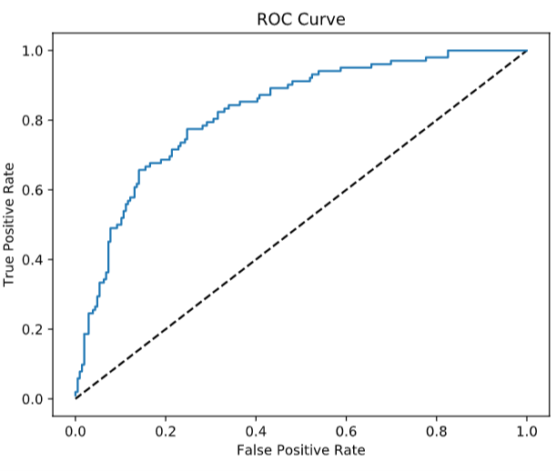
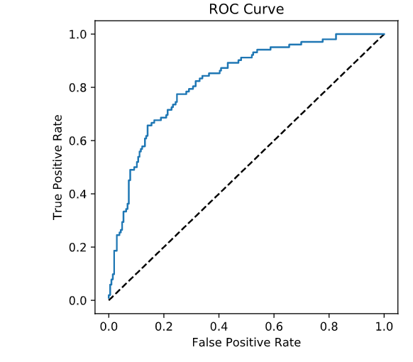
• ROC曲线是根据一系列不同的二分类方式（分界值或决定阈），以真正例率（也就是灵敏度recall）（True Positive Rate,TPR）为纵坐标，假正例率（1-特效性，）（False Positive Rate,FPR）为横坐标绘制的曲线。
• 要与混淆矩阵想结合

横轴FPR

\(\mathrm{FPR}=\frac{\mathrm{FP}}{\mathrm{FP}+\mathrm{TN}}\)
在所有真实值为Negative的数据中，被模型错误的判断为Positive的比例

如果两个概念熟，那就多看几遍

纵轴recall

这个好理解就是找回来
在所有真实值为Positive的数据中，被模型正确的判断为Positive的比例
\(\mathrm{TPR}=\frac{\mathrm{TP}}{\mathrm{TP}+\mathrm{FN}}\)

ROC曲线解读

• FPR与TPR分别构成了ROC曲线的横纵轴，因此我们知道在ROC曲线中，每一个点都对应着模型的一次结果

• 如果ROC曲线完全在纵轴上，代表这一点上，x=0，即FPR=0。模型没有把任何negative的数据错误的判为positive，预测完全准确
  不知道哪个大佬能做出来。。️

• 如果ROC曲线完全在横轴上，代表这一点上，y=0，即TPR=0。模型没有把任何positive的数据正确的判断为positive，预测完全不准确。
  平心而论，这种模型能做出来也是蛮牛的，因为模型真正做到了完全不准确，所以只要反着看结果就好了嘛

• 如果ROC曲线完全与右上方45度倾角线重合，证明模型的准确率是正好50%，错判的几率是一半一半

-因此，我们绘制出来ROC曲线的形状，是希望TPR大，而FPR小。因此对应在图上就是曲线尽量往左上角贴近。45度的直线一般被常用作Benchmark，即基准模型，我们的预测分类模型的ROC要能优于45度线，否则我们的预测还不如50/50的猜测来的准确

ROC曲线绘制

• ROC曲线上的一系列点，代表选取一系列的阈值（threshold）产生的结果
• 在分类问题中，我们模型预测的结果不是negative/positive。而是一个negatvie或positive的概率。那么在多大的概率下我们认为观测值应该是negative或positive呢？这个判定的值就是阈值（threshold）。
• ROC曲线上众多的点，每个点都对应着一个阈值的情况下模型的表现。多个点连起来就是ROC曲线了

API实现

sklearn.metrics.roc_curve(y_true,y_score,pos_label=None, sample_weight=None, drop_intermediate=True)

# Import the necessary modules
from sklearn.linear_model import LogisticRegression
from sklearn.metrics import confusion_matrix ,classification_report

# Create training and test sets
X_train, X_test, y_train, y_test = train_test_split(X, y, test_size = 0.4, random_state=42)

# Create the classifier: logreg
logreg = LogisticRegression()

# Fit the classifier to the training data
logreg.fit(X_train,y_train)

# Predict the labels of the test set: y_pred
y_pred = logreg.predict(X_test)

# Compute and print the confusion matrix and classification report
print(confusion_matrix(y_test, y_pred))
print(classification_report(y_test, y_pred))

# Import necessary modules
from sklearn.metrics import roc_curve

# Compute predicted probabilities: y_pred_prob
y_pred_prob = logreg.predict_proba(X_test)[:,1]

# Generate ROC curve values: fpr, tpr, thresholds
fpr, tpr, thresholds = roc_curve(y_test, y_pred_prob)

# Plot ROC curve
plt.plot([0, 1], [0, 1], 'k--')
plt.plot(fpr, tpr)
plt.xlabel('False Positive Rate')
plt.ylabel('True Positive Rate')
plt.title('ROC Curve')

AUC （Area under the ROC curve）

• AUC它就是值ROC曲线下的面积是多大。每一条ROC曲线对应一个AUC值。AUC的取值在0与1之间。
• AUC = 1，代表ROC曲线在纵轴上，预测完全准确。不管Threshold选什么，预测都是100%正确的。
• 0.5 < AUC < 1，代表ROC曲线在45度线上方，预测优于50/50的猜测。需要选择合适的阈值后，产出模型。
• AUC = 0.5，代表ROC曲线在45度线上，预测等于50/50的猜测。
• 0 < AUC < 0.5，代表ROC曲线在45度线下方，预测不如50/50的猜测。
• AUC = 0，代表ROC曲线在横轴上，预测完全不准确。

实现

sklearn.metrics.auc(x, y, reorder=False)

# Import necessary modules
from sklearn.model_selection import cross_val_score
from sklearn.metrics import roc_auc_score

# Compute predicted probabilities: y_pred_prob
y_pred_prob = logreg.predict_proba(X_test)[:,1]

# Compute and print AUC score
print("AUC: {}".format(roc_auc_score(y_test, y_pred_prob)))

# Compute cross-validated AUC scores: cv_auc
cv_auc = cross_val_score(logreg, X, y, cv=5, scoring='roc_auc')

# Print list of AUC scores
print("AUC scores computed using 5-fold cross-validation: {}".format(cv_auc))

<script.py> output:
    AUC: 0.8254806777079764
    AUC scores computed using 5-fold cross-validation: [0.80148148 0.8062963  0.81481481 0.86245283 0.8554717 ]

Precision-recall Curve

召回曲线也可以作为评估模型好坏的标准

• which is generated by plotting the precision and recall for different thresholds. As a reminder, precision and recall are defined as:
  Precision \(=\frac{T P}{T P+F P}\)
  Recall\(=\frac{T P}{T P+F N}\)

Hold-out set

模型评估之流出法

• 直接将数据集D划分为两个互斥的集合，其中一个集合作为训练集S，另外一个作为测试集T，即D=S∪T,S∩T=0.在S上训练出模型后，用T来评估其测试误差，作为对泛化误差的评估
• 训练/测试集的划分要尽可能的保持数据分布的一致性，避免因数据划分过程引入额外的偏差而对最终结果产生影响
• 在给定训练/测试集的样本比例后，仍然存在多种划分方式对初始数据集D进行划分，可能会对模型评估的结果产生影响。因此，单次使用留出法得到的结果往往不够稳定可靠，在使用留出法时，一般采用若干次随机划分、重复进行实验评估后取得平均值作为留出法的评估结果
• 此外。我们希望评估的是用D训练出的模型的性能，但是留出法需划分训练/测试集，这就会导致一个窘境：若另训练集S包含大多数的样本，则训练出的模型可能更接近于D训练出的模型，但是由于T比较小，评估结果可能不够稳定准确；若另测试集T包含多一些样本，则训练集S与D的差别更大，被评估的模型与用D训练出的模型相比可能就会有较大的误差，从而降低了评估结果的保真性（fidelity）。因此，常见的做法是：将大约2/3~4/5的样本用于训练，剩余样本作为测试参考

# Import necessary modules
from sklearn.model_selection import train_test_split
from sklearn.linear_model import LogisticRegression
from sklearn.model_selection import GridSearchCV

# Create the hyperparameter grid
c_space = np.logspace(-5, 8, 15)
param_grid = {'C': c_space, 'penalty': ['l1', 'l2']}

# Instantiate the logistic regression classifier: logreg
logreg = LogisticRegression()

# Create train and test sets
X_train, X_test, y_train, y_test = train_test_split(X, y, test_size = 0.4, random_state=42)

# Instantiate the GridSearchCV object: logreg_cv
logreg_cv = GridSearchCV(logreg, param_grid, cv=5)

# Fit it to the training data
logreg_cv.fit(X_train, y_train)

# Print the optimal parameters and best score
print("Tuned Logistic Regression Parameter: {}".format(logreg_cv.best_params_))
print("Tuned Logistic Regression Accuracy: {}".format(logreg_cv.best_score_))

<script.py> output:
    Tuned Logistic Regression Parameter: {'C': 0.4393970560760795, 'penalty': 'l1'}
    Tuned Logistic Regression Accuracy: 0.7652173913043478

# Import necessary modules
from sklearn.linear_model import ElasticNet
from sklearn.metrics import mean_squared_error
from sklearn.model_selection import GridSearchCV
from sklearn.model_selection import train_test_split

# Create train and test sets
X_train, X_test, y_train, y_test = train_test_split(X, y, test_size = 0.4, random_state=42)

# Create the hyperparameter grid
l1_space = np.linspace(0, 1, 30)
param_grid = {'l1_ratio': l1_space}

# Instantiate the ElasticNet regressor: elastic_net
elastic_net = ElasticNet()

# Setup the GridSearchCV object: gm_cv
gm_cv = GridSearchCV(elastic_net, param_grid, cv=5)

# Fit it to the training data
gm_cv.fit(X_train, y_train)

# Predict on the test set and compute metrics
y_pred = gm_cv.predict(X_test)
r2 = gm_cv.score(X_test, y_test)
mse = mean_squared_error(y_test, y_pred)
print("Tuned ElasticNet l1 ratio: {}".format(gm_cv.best_params_))
print("Tuned ElasticNet R squared: {}".format(r2))
print("Tuned ElasticNet MSE: {}".format(mse))

<script.py> output:
    Tuned ElasticNet l1 ratio: {'l1_ratio': 0.20689655172413793}
    Tuned ElasticNet R squared: 0.8668305372460283
    Tuned ElasticNet MSE: 10.05791413339844

classification_report（）

测试模型精度的方法很多，可以看下官方文档的例子，记一些常用的即可
API官方文档
https://scikit-learn.org/stable/modules/classes.html

MSE&RMSE

方差，标准差
MSE:\((y_真实-y_预测)^2\)之和
RMSE：MSE开平方

https://www.cnblogs.com/mindy-snail/p/12445973.html