2. Solving Linear Equations

2.1 Linear Equations Picture

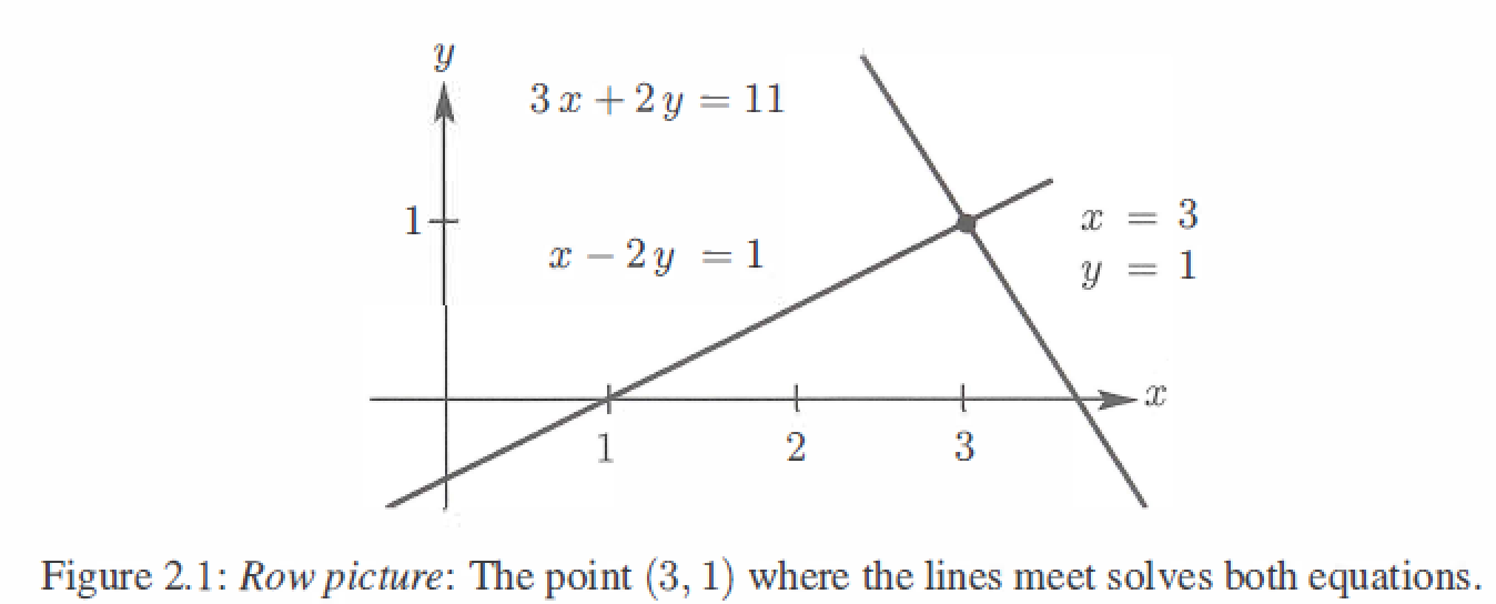
Row Picture

2 by 2 equations

Two equations, Two unknowns

\[\begin{matrix} x - 2y = 1 \\ 3x + 2y = 11 \end{matrix}
\]

The row picture shows two lines meeting at a single point(the solution).

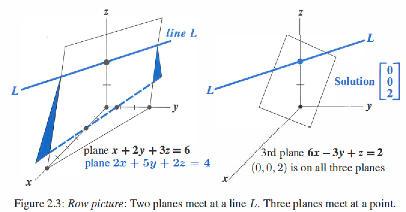
3 by 3 equations

Three equations, Three unknowns

\[Ax=b \ \ => \ \ \begin{matrix} x + 2y + 3z = 6 \\ 2x + 5y + 2z = 4 \\ 6x - 3y + z = 2\end{matrix}
\]

The row picture shows three planes meeting at a single point.

Column Picture

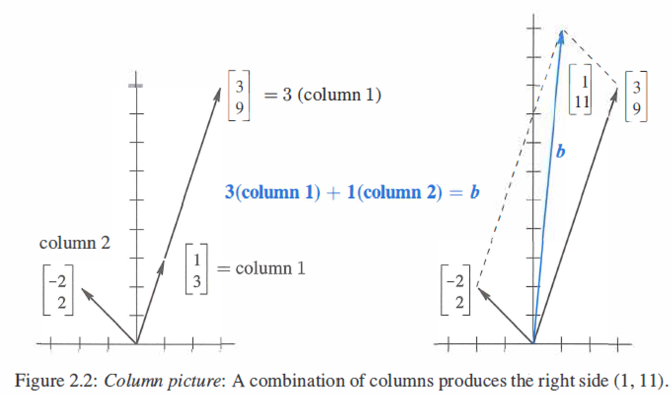
2 by 2 equations

Two equations, Two unknowns

\[\begin{matrix} x - 2y = 1 \\ 3x + 2y = 11 \end{matrix} =>x\left[ \begin{matrix} 1\\ 3 \\ \end{matrix} \right] + y\left[ \begin{matrix} -2\\ 2 \\ \end{matrix} \right] =\left[\begin{matrix} 1 \\ 11 \end{matrix}\right] = b
\]

The column picture combines the column vectors on the left side to produce the vector b on the right side.

(The left side of the vector equation is a linear combination of the columns)

3 by 3 equations

Three equations, Three unknowns

\[\begin{matrix} x + 2y + 3z = 6 \\ 2x + 5y + 2z = 4 \\ 6x - 3y + z = 2 \end{matrix} =>x\left[ \begin{matrix} 1\\ 2\\6 \\ \end{matrix} \right] + y\left[ \begin{matrix} 2\\ 5 \\-3 \\ \end{matrix} \right] + z\left[ \begin{matrix} 3\\ 2 \\1 \\ \end{matrix} \right] =\left[\begin{matrix} 4 \\ 6 \\ 2\end{matrix}\right] = b
\]

The column picture combines three columns to produce b，the coefficients (x,y,z) = (0,0,2).

2.2 Elimination

2.2.1 Gaussian Elimination

• Column 1 : Use the first equation to create zeros below the first pivot.
• Column 2 : Use the new equation 2 to create zeros below the second pivot.
• Column 3 to n : Keep going to find all n pivots and the upper triangular U.

2 by 2

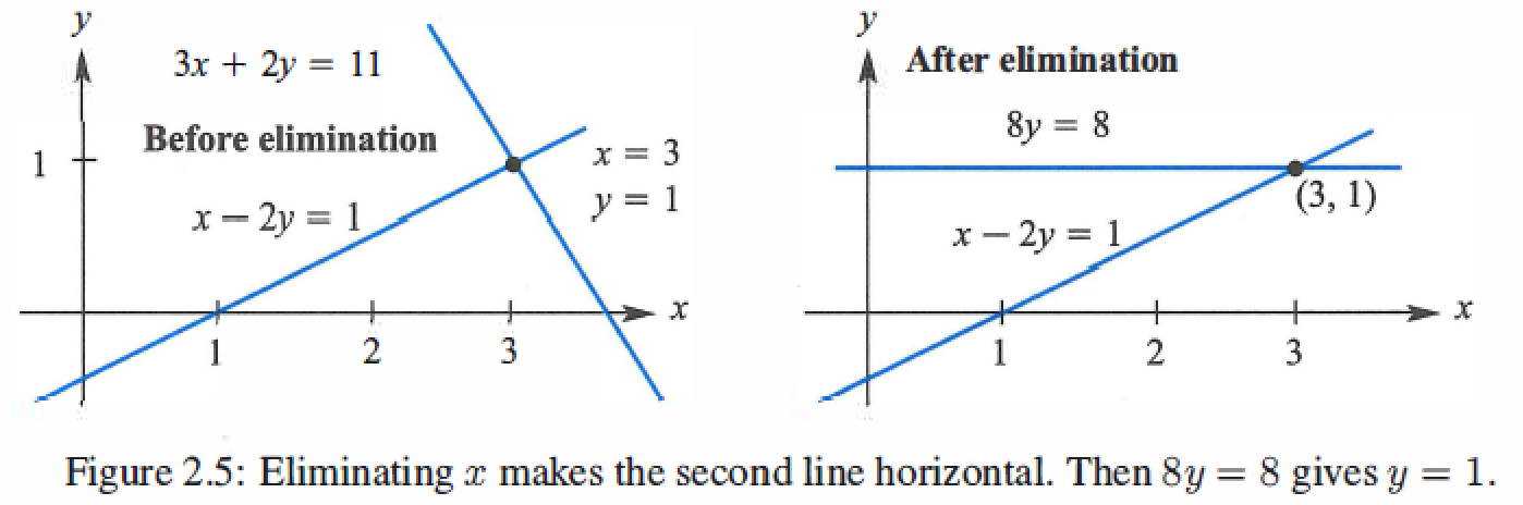
Multiply equation 1 by 3, and Subtract from equation 2.

\[(Before) \ \ \begin{matrix} x - 2y = 1 \\ 3x + 2y = 11 \end{matrix} ==> (After) \ \ \begin{matrix} x - 2y = 1 \\ 8y = 8 \end{matrix}
\]

3 by 3

\[Ax = b \ ==> \ \begin{matrix} 2x + 4y - 2z = 2 \\ 4x + 9y - 3z = 8 \\ -2x-3y+7z=10 \end{matrix}
\]

Elimination Steps

step1 : Subtract 2 times equation 1 from equation 2.

\[\begin{matrix} 2x + 4y - 2z = 2 \\
\quad \quad \quad y + z = 4 \\
-2x-3y+7z=10 \end{matrix}
\]

step2 : Subtract -1 times equation 1 from equation 3.

\[\begin{matrix} 2x + 4y - 2z = 2 \\
\quad \quad \quad y + z = 4 \\
\quad \quad \quad \quad y+5z=12 \end{matrix}
\]

step3 : Subtract new equation 2 from new equation 3.

\[\quad \begin{matrix} 2x + 4y - 2z = 2 \\
\quad \quad \quad \quad y + z = 4 \\
\quad \quad \quad \quad \quad 4z = 8 \end{matrix}
==>Ux = c
\]

U is upper triangular.

Back substitution

z = 2 --> y = 2 --> x = -1

2.2.2 Elimination-Matrix

Elimination multiplies Ax=b by \(E_{21} , E_{31} , E_{41}, ..., E_{n1}\), then \(E_{32} , E_{42}, ..., E_{n2}\) and onward.

• \(E =E_{21} ,..., E_{n1},..., E_{n2},...,E_{n(n-1)}\) , \(EA = [Ea_1...Ea_n]\)
• Augmented matrix : \(E[A\ \ b] = [EA\ \ Eb]\)

example:

\[Ax = b \\
\Downarrow \\
\begin{matrix} 2x_1 + 4x_2 - 2x_3 = 2 \\ 4x_1 + 9x_2 - 3x_3 = 8 \\ -2x_1-3x_2+7x_3=10 \end{matrix} \\
\Downarrow \\
\left[ \begin{matrix} 2&4&-2 \\ 4&9&-3 \\ -2&-3&7 \end{matrix} \right]
\left[ \begin{matrix} x_1\\x_2\\x_3 \end{matrix} \right] =
\left[ \begin{matrix} 2\\8\\10 \end{matrix} \right] \\
\Downarrow \\
\left[ \begin{matrix} 1&0&0 \\ -2&1&0 \\ 0&0&1 \end{matrix} \right]
\left[ \begin{matrix} 2&4&-2 \\ 4&9&-3 \\ -2&-3&7 \end{matrix} \right]
\left[ \begin{matrix} x_1\\x_2\\x_3 \end{matrix} \right] =
\left[ \begin{matrix} 1&0&0 \\ -2&1&0 \\ 0&0&1 \end{matrix} \right]
\left[ \begin{matrix} 2\\8\\10 \end{matrix} \right] \\
\Downarrow \\
\left[ \begin{matrix} 2&4&-2 \\ 0&1&1 \\ -2&-3&7 \end{matrix} \right]
\left[ \begin{matrix} x_1\\x_2\\x_3 \end{matrix} \right] =
\left[ \begin{matrix} 2\\4\\10 \end{matrix} \right] \\
\Downarrow \\
\left[ \begin{matrix} 1&0&0 \\ 0&1&0 \\ 1&0&1 \end{matrix} \right]
\left[ \begin{matrix} 2&4&-2 \\ 0&1&1 \\ -2&-3&7 \end{matrix} \right]
\left[ \begin{matrix} x_1\\x_2\\x_3 \end{matrix} \right] =
\left[ \begin{matrix} 1&0&0 \\ 0&1&0 \\ 1&0&1 \end{matrix} \right]
\left[ \begin{matrix} 2\\4\\10 \end{matrix} \right] \\
\Downarrow \\
\left[ \begin{matrix} 2&4&-2 \\ 0&1&1 \\ 0&1&5 \end{matrix} \right]
\left[ \begin{matrix} x_1\\x_2\\x_3 \end{matrix} \right] =
\left[ \begin{matrix} 2\\4\\12 \end{matrix} \right] \\
\Downarrow \\
\left[ \begin{matrix} 1&0&0 \\ 0&1&0 \\ 0&-1&1 \end{matrix} \right]
\left[ \begin{matrix} 2&4&-2 \\ 0&1&1 \\ 0&1&5 \end{matrix} \right]
\left[ \begin{matrix} x_1\\x_2\\x_3 \end{matrix} \right] =
\left[ \begin{matrix} 1&0&0 \\ 0&1&0 \\ 0&-1&1 \end{matrix} \right]
\left[ \begin{matrix} 2\\4\\12 \end{matrix} \right] \\
\Downarrow \\
\left[ \begin{matrix} 2&4&-2 \\ 0&1&1 \\ 0&0&4 \end{matrix} \right]
\left[ \begin{matrix} x_1\\x_2\\x_3 \end{matrix} \right] =
\left[ \begin{matrix} 2\\4\\8 \end{matrix} \right] \\
\Downarrow Back \ \ substitution \\
x_3 = 2 , x_2 = 2, x_1 = -1
\]

2.3 Rules for Matrix Operations

2.3.1 Matrix Multiplication

Matrices A with n columns multiply matrices B with n rows : \(A_{m \times n} B_{n \times p} = C_{m \times p}\)

The regular way

The entry in row i and column j of AB is (row i of A) \(\cdot\) (column j of B): \((AB)_{ij}=a_{i1}b_{1j} + a_{i2}b_{2j}+...+a_{in}b_{nj}\)

\[\left[ \begin{matrix} * \\ a_{i1}&a_{i2}&...&a_{in} \\ * \\* \end{matrix} \right]
\left[ \begin{matrix} *&b_{1j}&*&*\\ &b_{2j}&&\ \\ &\vdots&& \\ &b_{nj}&& \end{matrix} \right]=
\left[ \begin{matrix} &&*&& \\ *&*&(AB)_{ij}&*&* \\ &&*&& \\&&*&& \end{matrix} \right]
\]

The column way

Each column of AB is a combination of the columns of A.

Matrix A times every column of B : \(A[b_1...b_p]=[Ab_1...Ab_p]\)

The row way

Every row of AB is a combination of the rows of B

Every row of A times matrix B : \(\left[\begin{matrix} a_1 \\ a_2 \\ \vdots \\a_n \end{matrix}\right]B=\left[\begin{matrix} a_1B \\ a_2B \\ \vdots \\a_nB \end{matrix}\right]\)

The columns multiply rows

Multiply columns 1 to n of A times rows 1 to n of B. Add those matrices.

\[\left[\begin{matrix} col_1&\cdots&col_n \\ \vdots&\vdots&\vdots \end{matrix}\right]
\left[\begin{matrix} row_1&\cdots \\ \vdots&\vdots \\row_n&\cdots \end{matrix}\right]
=(col_1)(row_1)+...+(col_n)(row_n)
\]

Block Multiplication

A and B cut into blocks(which are small matrices).

\[A = \left[\begin{matrix} A_1&A_2\\ A_3&A_4 \end{matrix}\right] \\
B = \left[\begin{matrix} B_1&B_2\\ B_3&B_4 \end{matrix}\right] \\
AB =\left[\begin{matrix} A_1&A_2\\ A_3&A_4 \end{matrix}\right]
\left[\begin{matrix} B_1&B_2\\ B_3&B_4 \end{matrix}\right] =
\left[\begin{matrix} A_1B_1 + A_2B_3&A_1B_2 + A_2B_4\\ A_3B_1 + A_4B_3&A_2B_2 + A_4B_4\end{matrix}\right]
\]

2.3.2 The Laws for Matrix Operations

Additions

Commutative law : A + B = B + A

Distributive law : c(A + B) = cA + cB

Associative law : A + (B + C) = (A + B) + C

Multiply

Commutative law is usually broken : \(AB \neq BA\)

Distributive law : (A + B)C = AC + BC or C(A + B) = CA + CB

Associative law : A (B C) = (A B) C

2.4 Inverse Matrices

The matrix A is invertible if there exists a matrix \(A^{-1}\) that "inverts" A :

\[A^{-1}A = I \quad and \quad AA^{-1}=I
\]

• A is invertible if and only if it has n pivots (row exchanges allowed).
• If Ax = 0 for a nonzero vector x, then A has no inverse.
• The inverse of AB is the reverse product \(B^{-1}A^{-1}\)，and \((ABC)^{-1}=C^{-1}B^{-1}A^{-1}\).
• Diagonally dominant matrices are invertible.Each \(|a_{ii}|\)dominates its row.

Gauss-Jordan Method

\[[A \quad I] \quad reduce \quad to \quad [I \quad A^{-1}]
\]

example $A = \left[ \begin{matrix} 2&3 \ 4&7 \end{matrix}\right] $:

\[[A \quad I] = \left[ \begin{matrix} 2&3&1&0 \\ 4&7&0&1 \end{matrix}\right] \\
\Downarrow \\
[U \quad L^{-1}]=\left[ \begin{matrix} 2&3&1&0 \\ 0&1&-2&1 \end{matrix}\right] \quad \\
\Downarrow \\
\left[ \begin{matrix} 2&0&7&-3 \\ 0&1&-2&1 \end{matrix}\right] \\
\Downarrow \\
[I \quad A^{-1}]=\left[ \begin{matrix} 1&0&7/2&-3/2 \\ 0&1&-2&1 \end{matrix}\right] \quad \\
\]

2.5 Factorization : A = LU

Gaussian elimination (with no row exchanges) factors A into L times U，the factors L and U are triangular matrices, and L include all their inverse.

\[A = LU \quad (which \quad L \rightarrow lower \quad triangular, \quad U \rightarrow upper \quad trangular)
\]

\[(E_{n(n-1)}...E_{31}E_{21})A = U \\
\Downarrow \\
(E_{21}^{-1}E_{31}^{-1}...E_{n(n-1)}^{-1})(E_{n(n-1)}...E_{31}E_{21})A = (E_{21}^{-1}E_{31}^{-1}...E_{n(n-1)}^{-1})U \\
\Downarrow \\
A = LU \\
\]

example \(A = \left[ \begin{matrix} 2&1&0 \\ 1&2&1 \\ 0&1&2 \end{matrix}\right] =
\left[ \begin{matrix} 1&0&0 \\ 1/2&1&0 \\ 0&2/3&1 \end{matrix}\right]
\left[ \begin{matrix} 2&1&0 \\ 0&3/2&1 \\ 0&0&4/3 \end{matrix}\right] = LU\)

The triangular factorization can be written : \(A = LU \rightarrow A=LDU\), that D is a diagonal matrix contains the pivots.

Split U into \(DU=\left[ \begin{matrix} d_1&&& \\ &d_2&& \\ &&\ddots \\ &&&d_n \end{matrix}\right]\left[ \begin{matrix} 1&u_{12}/d_1&u_{13}/d_1&\cdots \\ &1&u_{23}/d_2&\vdots \\ &&\ddots \\ &&&1 \end{matrix}\right]\)

example:

\[A = \left[ \begin{matrix} 2&1&0 \\ 1&2&1 \\ 0&1&2 \end{matrix}\right] \\ =
\left[ \begin{matrix} 1&0&0 \\ 1/2&1&0 \\ 0&2/3&1 \end{matrix}\right]
\left[ \begin{matrix} 2&1&0 \\ 0&3/2&1 \\ 0&0&4/3 \end{matrix}\right] \\ =
\left[ \begin{matrix} 1&0&0 \\ 1/2&1&0 \\ 0&2/3&1 \end{matrix}\right]
\left[ \begin{matrix} 2&0&0 \\ 0&3/2&0 \\ 0&0&4/3 \end{matrix}\right]\left[ \begin{matrix} 1&1/2&0 \\ 0&1&2/3 \\ 0&0&1 \end{matrix}\right]= LDU
\]

Keys

• The lower triangular L contains the number \(l_{ij}\) that multiply pivot rows, going from A to U. The product LU adds those rows back to recover A.
• On the right side we solve Lc = b (forward) and Ux=c (backward).
• Cost : the left side costs \(1/3(n^3 -n)\) multiplications and subtractions，the right side costs \(n^2\) multiplications and subtractions.

2.6 Transposes and Permutations

Transposes

The columns of \(A^{T}\) are the rows of A

\[(A^{T})_{ij} = A_{ji}
\]

If \(A = \left [ \begin{matrix} 1&2&3 \\ 0&0&4 \end{matrix}\right]\) then \(A^{T} = \left [ \begin{matrix} 1&0 \\ 2&0 \\ 3&4 \end{matrix}\right]\)

Sum : \((A+B)^{T} = A^{T} + B^{T}\)

Product : \((AB)^{T} = B^{T}A^{T}\)

Inverse : \((A^{T})^{-1} = (A^{-1})^{T}\)

Symmetric matrix (\(S^T=S\))：\(U = L^T \rightarrow S = LDU = LDL^T\)

Permutations

A permutation matrix P has the rows of the identity I in any order, \(P_{ij}\) is constructed by exchanging two row i and j of \(I\)，and there are \(n!\) permuataion matrices of order n.

3 by 3 permuation matrices:

\[I = \left [ \begin{matrix} 1&& \\ &1& \\ &&1 \end{matrix}\right] \quad
P_{21} = \left [ \begin{matrix} &1& \\ 1&& \\ &&1 \end{matrix}\right] \quad
P_{31} = \left [ \begin{matrix} &&1\\ &1& \\ 1&& \end{matrix}\right] \\
P_{32} = \left [ \begin{matrix} 1&&\\ &&1 \\ &1& \end{matrix}\right] \quad
P_{32}P_{21} = \left [ \begin{matrix} &1&\\ &&1 \\ 1&& \end{matrix}\right] \quad
P_{21}P_{32} = \left [ \begin{matrix} &&1\\ 1&& \\ &1& \end{matrix}\right]
\]

• If A is invertible then a permutation P will reorder its rows for PA=LU.
• A permutation matrix P has a 1 in each row and column, and \(P^T = P^{-1}\).