Zipline入门教程

Zipline Beginner Tutorial

Basics 基础

Zipline is an open-source algorithmic trading simulator written in Python. Zipline是开源的算法交易模拟器，使用python编写。

The source can be found at: https://github.com/quantopian/zipline

Some benefits include:

• Realistic: slippage, transaction costs, order delays.
• Stream-based: Process each event individually, avoids look-ahead bias.
• Batteries included: Common transforms (moving average) as well as common risk calculations (Sharpe).
• Developed and continuously updated by Quantopian which provides an easy-to-use web-interface to Zipline, 10 years of minute-resolution historical US stock data, and live-trading capabilities. This tutorial is directed at users wishing to use Zipline without using Quantopian. If you instead want to get started on Quantopian, see here.

This tutorial assumes that you have zipline correctly installed, see the installation instructions if you haven’t set up zipline yet.

Every zipline algorithm consists of two functions you have to define: 每一个zipline算法由以下2个函数组成，

initialize(context)
handle_data(context, data)

Before the start of the algorithm, zipline calls the initialize() function and passes in a context variable. context is a persistent namespace for you to store variables you need to access from one algorithm iteration to the next.

在算法启动之前，zipline调用initialize()函数，并传入变量context。context是个持久的命名空间，用于存储需要的变量，你可以将其迭代到其他算法中。

After the algorithm has been initialized, zipline calls the handle_data() function once for each event. At every call, it passes the same context variable and an event-frame called data containing the current trading bar with open, high, low, and close (OHLC) prices as well as volume for each stock in your universe. For more information on these functions, see the relevant part of the Quantopian docs.

算法初始化之后，zipline为每个事件调用handle_data()函数一次，每次调用之后，它传递相同的context变量以及一个叫data的事件框架，其中包含当前交易条(OHLCV数据)。

My first algorithm 第一个算法

Lets take a look at a very simple algorithm from the examples directory, buyapple.py:

from zipline.examples import buyapple
buyapple??

from zipline.api import order, record, symbol

def initialize(context):
    pass

def handle_data(context, data):
    order(symbol('AAPL'), 10)
    record(AAPL=data.current(symbol('AAPL'), 'price'))

As you can see, we first have to import some functions we would like to use. All functions commonly used in your algorithm can be found in zipline.api. Here we are using order() which takes two arguments: a security object, and a number specifying how many stocks you would like to order (if negative, order() will sell/short stocks). In this case we want to order 10 shares of Apple at each iteration. For more documentation on order(), see the Quantopian docs.

order()带了2个参数：对象和购买股数(负表示卖出)，此例中要在每次迭代中买入10股苹果

Finally, the record() function allows you to save the value of a variable at each iteration. You provide it with a name for the variable together with the variable itself: varname=var. After the algorithm finished running you will have access to each variable value you tracked with record() under the name you provided (we will see this further below). You also see how we can access the current price data of the AAPL stock in the data event frame (for more information see here.

Running the algorithm 运行

To now test this algorithm on financial data, zipline provides three interfaces: A command-line interface, IPython Notebook magic, and run_algorithm().

Ingesting Data 导入数据

If you haven’t ingested the data, run:

$ zipline ingest [-b <bundle>]

where <bundle> is the name of the bundle to ingest, defaulting to quantopian-quandl.

you can check out the ingesting data section for more detail.

Command line interface

After you installed zipline you should be able to execute the following from your command line (e.g. cmd.exe on Windows, or the Terminal app on OSX):

$ zipline run --help

Usage: zipline run [OPTIONS]

  Run a backtest for the given algorithm.

Options:
  -f, --algofile FILENAME         The file that contains the algorithm to run.
  -t, --algotext TEXT             The algorithm script to run.
  -D, --define TEXT               Define a name to be bound in the namespace
                                  before executing the algotext. For example
                                  '-Dname=value'. The value may be any python
                                  expression. These are evaluated in order so
                                  they may refer to previously defined names.
  --data-frequency [minute|daily]
                                  The data frequency of the simulation.
                                  [default: daily]
  --capital-base FLOAT            The starting capital for the simulation.
                                  [default: 10000000.0]
  -b, --bundle BUNDLE-NAME        The data bundle to use for the simulation.
                                  [default: quantopian-quandl]
  --bundle-timestamp TIMESTAMP    The date to lookup data on or before.
                                  [default: <current-time>]
  -s, --start DATE                The start date of the simulation.
  -e, --end DATE                  The end date of the simulation.
  -o, --output FILENAME           The location to write the perf data. If this
                                  is '-' the perf will be written to stdout.
                                  [default: -]
  --print-algo / --no-print-algo  Print the algorithm to stdout.
  --help                          Show this message and exit.

As you can see there are a couple of flags that specify where to find your algorithm (-f) as well as parameters specifying which data to use, defaulting to the Quantopian Quandl WIKI Mirror. There are also arguments for the date range to run the algorithm over (--start and --end). Finally, you’ll want to save the performance metrics of your algorithm so that you can analyze how it performed. This is done via the --output flag and will cause it to write the performance DataFrame in the pickle Python file format. Note that you can also define a configuration file with these parameters that you can then conveniently pass to the -c option so that you don’t have to supply the command line args all the time (see the .conf files in the examples directory).

Thus, to execute our algorithm from above and save the results to buyapple_out.pickle we would call zipline run as follows:

zipline run -f ../../zipline/examples/buyapple.py --start -- --end -- -o buyapple_out.pickle

AAPL
[-- :: trading days out of .
[-- ::-- ::+:
[-- ::-- ::+:

run first calls the initialize() function, and then streams the historical stock price day-by-day through handle_data(). After each call to handle_data() we instruct zipline to order 10 stocks of AAPL. After the call of the order() function, zipline enters the ordered stock and amount in the order book. After the handle_data() function has finished, zipline looks for any open orders and tries to fill them. If the trading volume is high enough for this stock, the order is executed after adding the commission and applying the slippage model which models the influence of your order on the stock price, so your algorithm will be charged more than just the stock price * 10. (Note, that you can also change the commission and slippage model that zipline uses, see the Quantopian docs for more information).

Lets take a quick look at the performance DataFrame. For this, we use pandas from inside the IPython Notebook and print the first ten rows. Note that zipline makes heavy usage of pandas, especially for data input and outputting so it’s worth spending some time to learn it.

import pandas as pd
perf = pd.read_pickle('buyapple_out.pickle') # read in perf DataFrame
perf.head()

	AAPL	algo_volatility	algorithm_period_return	alpha	benchmark_period_return	benchmark_volatility	beta	capital_used	ending_cash	ending_exposure	...	short_exposure	short_value	shorts_count	sortino	starting_cash	starting_exposure	starting_value	trading_days	transactions	treasury_period_return
2000-01-03 21:00:00	3.738314	0.000000e+00	0.000000e+00	-0.065800	-0.009549	0.000000	0.000000	0.00000	10000000.00000	0.00000	...	0	0	0	0.000000	10000000.00000	0.00000	0.00000	1	[]	0.0658
2000-01-04 21:00:00	3.423135	3.367492e-07	-3.000000e-08	-0.064897	-0.047528	0.323229	0.000001	-34.53135	9999965.46865	34.23135	...	0	0	0	0.000000	10000000.00000	0.00000	0.00000	2	[{u'order_id': u'513357725cb64a539e3dd02b47da7...	0.0649
2000-01-05 21:00:00	3.473229	4.001918e-07	-9.906000e-09	-0.066196	-0.045697	0.329321	0.000001	-35.03229	9999930.43636	69.46458	...	0	0	0	0.000000	9999965.46865	34.23135	34.23135	3	[{u'order_id': u'd7d4ad03cfec4d578c0d817dc3829...	0.0662
2000-01-06 21:00:00	3.172661	4.993979e-06	-6.410420e-07	-0.065758	-0.044785	0.298325	-0.000006	-32.02661	9999898.40975	95.17983	...	0	0	0	-12731.780516	9999930.43636	69.46458	69.46458	4	[{u'order_id': u'1fbf5e9bfd7c4d9cb2e8383e1085e...	0.0657
2000-01-07 21:00:00	3.322945	5.977002e-06	-2.201900e-07	-0.065206	-0.018908	0.375301	0.000005	-33.52945	9999864.88030	132.91780	...	0	0	0	-12629.274583	9999898.40975	95.17983	95.17983	5	[{u'order_id': u'9ea6b142ff09466b9113331a37437...	0.0652

5 rows × 39 columns

As you can see, there is a row for each trading day, starting on the first business day of 2000. In the columns you can find various information about the state of your algorithm. The very first columnAAPL was placed there by the record() function mentioned earlier and allows us to plot the price of apple. For example, we could easily examine now how our portfolio value changed over time compared to the AAPL stock price.

%pylab inline
figsize(12, 12)
import matplotlib.pyplot as plt

ax1 = plt.subplot(211)
perf.portfolio_value.plot(ax=ax1)
ax1.set_ylabel('portfolio value')
ax2 = plt.subplot(212, sharex=ax1)
perf.AAPL.plot(ax=ax2)
ax2.set_ylabel('AAPL stock price')

Populating the interactive namespace from numpy and matplotlib

<matplotlib.text.Text at 0x7ff5c6147f90>

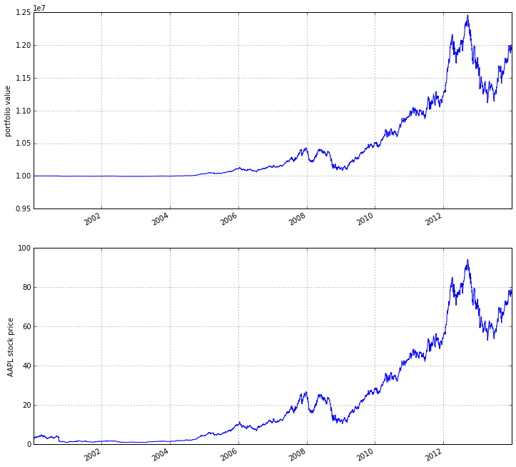
As you can see, our algorithm performance as assessed by the portfolio_value closely matches that of the AAPL stock price. This is not surprising as our algorithm only bought AAPL every chance it got.

IPython Notebook

The IPython Notebook is a very powerful browser-based interface to a Python interpreter (this tutorial was written in it). As it is already the de-facto interface for most quantitative researchers zipline provides an easy way to run your algorithm inside the Notebook without requiring you to use the CLI.

To use it you have to write your algorithm in a cell and let zipline know that it is supposed to run this algorithm. This is done via the %%zipline IPython magic command that is available after youimport zipline from within the IPython Notebook. This magic takes the same arguments as the command line interface described above. Thus to run the algorithm from above with the same parameters we just have to execute the following cell after importing zipline to register the magic.

%load_ext zipline

%%zipline --start 2000-1-1 --end 2014-1-1
from zipline.api import symbol, order, record

def initialize(context):
    pass

def handle_data(context, data):
    order(symbol('AAPL'), 10)
    record(AAPL=data[symbol('AAPL')].price)

Note that we did not have to specify an input file as above since the magic will use the contents of the cell and look for your algorithm functions there. Also, instead of defining an output file we are specifying a variable name with -o that will be created in the name space and contain the performance DataFrame we looked at above.

_.head()

	AAPL	algo_volatility	algorithm_period_return	alpha	benchmark_period_return	benchmark_volatility	beta	capital_used	ending_cash	ending_exposure	...	short_exposure	short_value	shorts_count	sortino	starting_cash	starting_exposure	starting_value	trading_days	transactions	treasury_period_return
2000-01-03 21:00:00	3.738314	0.000000e+00	0.000000e+00	-0.065800	-0.009549	0.000000	0.000000	0.00000	10000000.00000	0.00000	...	0	0	0	0.000000	10000000.00000	0.00000	0.00000	1	[]	0.0658
2000-01-04 21:00:00	3.423135	3.367492e-07	-3.000000e-08	-0.064897	-0.047528	0.323229	0.000001	-34.53135	9999965.46865	34.23135	...	0	0	0	0.000000	10000000.00000	0.00000	0.00000	2	[{u'commission': 0.3, u'amount': 10, u'sid': 0...	0.0649
2000-01-05 21:00:00	3.473229	4.001918e-07	-9.906000e-09	-0.066196	-0.045697	0.329321	0.000001	-35.03229	9999930.43636	69.46458	...	0	0	0	0.000000	9999965.46865	34.23135	34.23135	3	[{u'commission': 0.3, u'amount': 10, u'sid': 0...	0.0662
2000-01-06 21:00:00	3.172661	4.993979e-06	-6.410420e-07	-0.065758	-0.044785	0.298325	-0.000006	-32.02661	9999898.40975	95.17983	...	0	0	0	-12731.780516	9999930.43636	69.46458	69.46458	4	[{u'commission': 0.3, u'amount': 10, u'sid': 0...	0.0657
2000-01-07 21:00:00	3.322945	5.977002e-06	-2.201900e-07	-0.065206	-0.018908	0.375301	0.000005	-33.52945	9999864.88030	132.91780	...	0	0	0	-12629.274583	9999898.40975	95.17983	95.17983	5	[{u'commission': 0.3, u'amount': 10, u'sid': 0...	0.0652

5 rows × 39 columns

Access to previous prices using history

Working example: Dual Moving Average Cross-Over 双移动平均线交叉

The Dual Moving Average (DMA) is a classic momentum strategy. It’s probably not used by any serious trader anymore but is still very instructive. The basic idea is that we compute two rolling or moving averages (mavg) – one with a longer window that is supposed to capture long-term trends and one shorter window that is supposed to capture short-term trends. Once the short-mavg crosses the long-mavg from below we assume that the stock price has upwards momentum and long the stock. If the short-mavg crosses from above we exit the positions as we assume the stock to go down further.

As we need to have access to previous prices to implement this strategy we need a new concept: History

data.history() is a convenience function that keeps a rolling window of data for you. The first argument is the number of bars you want to collect, the second argument is the unit (either '1d' for '1m' but note that you need to have minute-level data for using 1m). For a more detailed description history()‘s features, see the Quantopian docs. Let’s look at the strategy which should make this clear:

%%zipline --start 2000-1-1 --end 2012-1-1 -o dma.pickle

from zipline.api import order_target, record, symbol

def initialize(context):
    context.i = 0
    context.asset = symbol('AAPL')

def handle_data(context, data):
    # Skip first 300 days to get full windows
    context.i += 1
    if context.i < 300:
        return

    # Compute averages
    # data.history() has to be called with the same params
    # from above and returns a pandas dataframe.
    short_mavg = data.history(context.asset, 'price', bar_count=100, frequency="1d").mean()
    long_mavg = data.history(context.asset, 'price', bar_count=300, frequency="1d").mean()

    # Trading logic
    if short_mavg > long_mavg:
        # order_target orders as many shares as needed to
        # achieve the desired number of shares.
        order_target(context.asset, 100)
    elif short_mavg < long_mavg:
        order_target(context.asset, 0)

    # Save values for later inspection
    record(AAPL=data.current(context.asset, 'price'),
           short_mavg=short_mavg,
           long_mavg=long_mavg)

def analyze(context, perf):
    fig = plt.figure()
    ax1 = fig.add_subplot(211)
    perf.portfolio_value.plot(ax=ax1)
    ax1.set_ylabel('portfolio value in $')

    ax2 = fig.add_subplot(212)
    perf['AAPL'].plot(ax=ax2)
    perf[['short_mavg', 'long_mavg']].plot(ax=ax2)

    perf_trans = perf.ix[[t != [] for t in perf.transactions]]
    buys = perf_trans.ix[[t[0]['amount'] > 0 for t in perf_trans.transactions]]
    sells = perf_trans.ix[
        [t[0]['amount'] < 0 for t in perf_trans.transactions]]
    ax2.plot(buys.index, perf.short_mavg.ix[buys.index],
             '^', markersize=10, color='m')
    ax2.plot(sells.index, perf.short_mavg.ix[sells.index],
             'v', markersize=10, color='k')
    ax2.set_ylabel('price in $')
    plt.legend(loc=0)
    plt.show()

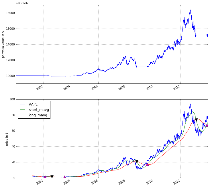
Here we are explicitly defining an analyze() function that gets automatically called once the backtest is done (this is not possible on Quantopian currently).

Although it might not be directly apparent, the power of history() (pun intended) can not be under-estimated as most algorithms make use of prior market developments in one form or another. You could easily devise a strategy that trains a classifier with scikit-learn which tries to predict future market movements based on past prices (note, that most of the scikit-learn functions require numpy.ndarrays rather than pandas.DataFrames, so you can simply pass the underlying ndarray of a DataFrame via .values).

We also used the order_target() function above. This and other functions like it can make order management and portfolio rebalancing much easier. See the Quantopian documentation on order functions fore more details.

Conclusions

We hope that this tutorial gave you a little insight into the architecture, API, and features of zipline. For next steps, check out some of the examples.

Feel free to ask questions on our mailing list, report problems on our GitHub issue tracker, get involved, and checkout Quantopian.