
XGBOOST应用及调参示例
该示例所用的数据可从该链接下载,提取码为3y90,数据说明可参考该网页。该示例的“模型调参”这一部分引用了这篇博客的步骤。
数据前处理
- 导入数据
import pandas as pd

import numpy as np

from sklearn.cross_validation import train_test_split

### Load data

### Split the data to train and test sets

data = pd.read_csv('data/loan/Train.csv', encoding = "ISO-8859-1")

train, test = train_test_split(data,train_size=0.7,random_state=123,stratify=data['Disbursed'])

### Check number of nulls in each feature column

nulls_per_column = train.isnull().sum()

print(nulls_per_column) - 将特征拆分成数值型和种类型
### Drop the useless columns

train_1 = train.drop(['ID','Lead_Creation_Date','LoggedIn'],axis=1)

### Split the columns to numerical and categorical

category_cols = train_1.columns[train_1.dtypes==object].tolist()

category_cols.remove('DOB')

category_cols.append('Var4')

numeric_cols = list(set(train_1.columns)-set(category_cols)) - 分析并处理种类型特征
### explore the categorical columns

for v in category_cols:

    print('Ratio of missing value for variable {0}: {1}'.format(v,nulls_per_column[v]/train_1.shape[0]))

print('-----------------------------------------------------------')

counts = dict()

for v in category_cols:

    print('\nFrequency count for variable %s'%v)

    counts[v] = train_1[v].value_counts()

    print(counts[v])

### merge the cities that counts<200

merge_city = [c for c in counts['City'].index if counts['City'][c]<200]

train_1['City'] = train_1['City'].apply(lambda x: 'others' if x in merge_city else x)

### merge the salary accounts that counts<100

merge_sa = [c for c in counts['Salary_Account'].index if counts['Salary_Account'][c]<100]

train_1['Salary_Account'] = train_1['Salary_Account'].apply(lambda x: 'others' if x in merge_sa else x)

### merge the sources that counts<100

merge_sr = [c for c in counts['Source'].index if counts['Source'][c]<100]

train_1['Source'] = train_1['Source'].apply(lambda x: 'others' if x in merge_sr else x)

### impute the missing value

train_1['City'].fillna('Missing',inplace=True)

train_1['Salary_Account'].fillna('Missing',inplace=True)

### delete the column Employer_Name since too many categories

train_2 = train_1.drop('Employer_Name',axis=1) - 分析并处理数值型特征
### Explore the numerical columns

for v in numeric_cols:

    print('Ratio of missing value for variable {0}: {1}'.format(v,nulls_per_column[v]/train_2.shape[0]))

print('-----------------------------------------------------------')

for v in numeric_cols:

    print('\nStatistical summary for variable %s'%v)

    print(train_2[v].describe())

### Create Age column:

train_2['Age'] = train_2['DOB'].apply(lambda x: 118 - int(x[-2:]))

### High proportion missing so create a new variable stating whether this is missing or not:

train_2['Loan_Amount_Submitted_Missing'] = train_2['Loan_Amount_Submitted'].apply(lambda x: 1 if pd.isnull(x) else 0)

train_2['Loan_Tenure_Submitted_Missing'] = train_2['Loan_Tenure_Submitted'].apply(lambda x: 1 if pd.isnull(x) else 0)

train_2['EMI_Loan_Submitted_Missing'] = train_2['EMI_Loan_Submitted'].apply(lambda x: 1 if pd.isnull(x) else 0)

train_2['Interest_Rate_Missing'] = train_2['Interest_Rate'].apply(lambda x: 1 if pd.isnull(x) else 0)

train_2['Processing_Fee_Missing'] = train_2['Processing_Fee'].apply(lambda x: 1 if pd.isnull(x) else 0)

### Impute the missing value

train_2['Existing_EMI'].fillna(train_2['Existing_EMI'].median(), inplace=True)

train_2['Loan_Amount_Applied'].fillna(train_2['Loan_Amount_Applied'].median(),inplace=True)

train_2['Loan_Tenure_Applied'].fillna(train_2['Loan_Tenure_Applied'].median(),inplace=True)

### Drop original columns

train_3 = train_2.drop(['DOB','Loan_Amount_Submitted','Loan_Tenure_Submitted','EMI_Loan_Submitted', \

'Interest_Rate','Processing_Fee'],axis=1) - One-Hot encoding
from sklearn.preprocessing import LabelEncoder

dropped_columns = ['ID','Lead_Creation_Date','LoggedIn','Employer_Name','DOB','Loan_Amount_Submitted', \

                'Loan_Tenure_Submitted','EMI_Loan_Submitted','Interest_Rate','Processing_Fee']

le = LabelEncoder()

var_to_encode = list(set(category_cols)-set(dropped_columns))

for col in var_to_encode:

    train_3[col] = le.fit_transform(train_3[col])

### pd.get_dummies can also be used directly without LabelEncoder

train_3 = pd.get_dummies(train_3, columns=var_to_encode)
模型调参
- 建立基础模型并使用early_stop调整迭代次数
import xgboost as xgb

import matplotlib.pyplot as plt

from sklearn import metrics

### base model

target = 'Disbursed'

predictors = [x for x in train_3.columns if x!=target]

xgb1 = xgb.XGBClassifier(learning_rate=0.1, n_estimators=1000, max_depth=5, min_child_weight=1, gamma=0, \

                         subsample=0.8, colsample_bytree=0.8, objective= 'binary:logistic', nthread=4, seed=27)

### use early_stop in xgb.cv

def get_n_estimators(alg, dtrain, predictors, target, cv_folds=5, early_stopping_rounds=50):

    xgb_param = alg.get_xgb_params()

    xgtrain = xgb.DMatrix(dtrain[predictors], label=dtrain[target])

    cvresult = xgb.cv(xgb_param, xgtrain, num_boost_round=alg.get_params()['n_estimators'], nfold=cv_folds, \

                      metrics='auc', early_stopping_rounds=early_stopping_rounds, stratified=True)

    alg.set_params(n_estimators=cvresult.shape[0])

    #Print model report:

    print("\nModel Report")

    print("Set n_estimators to {0}".format(cvresult.shape[0]))

    print(cvresult.tail(1)['test-auc-mean'])

    #Fit the algorithm on the data

    alg.fit(dtrain[predictors], dtrain[target], eval_metric='auc')

    #Feature importance

    feat_imp = pd.Series(alg.get_booster().get_fscore()).sort_values(ascending=False)

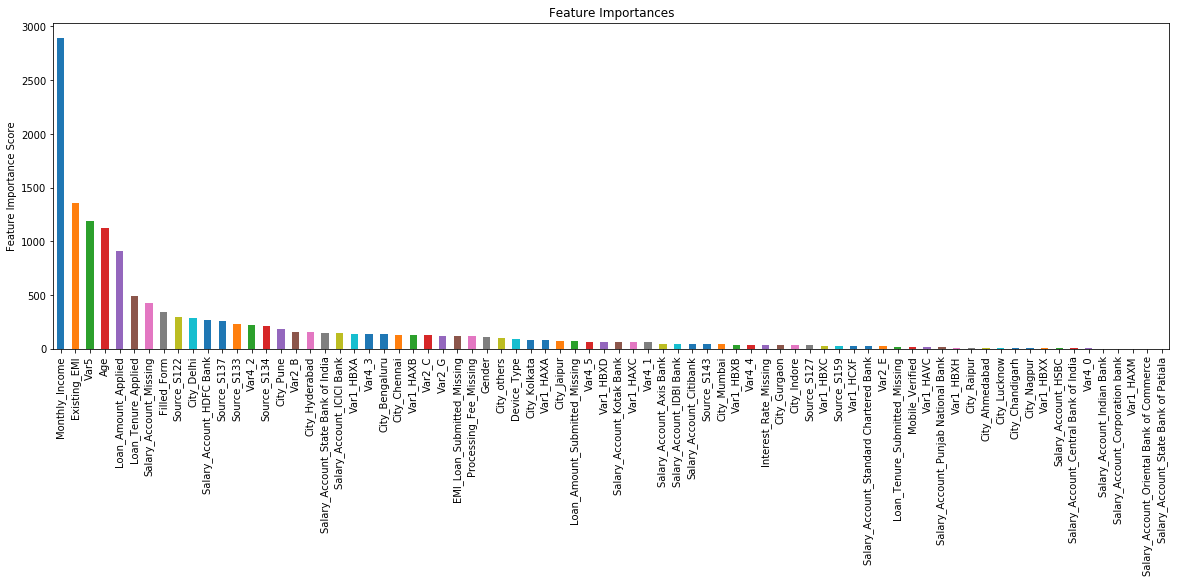
    feat_imp.plot(kind='bar', title='Feature Importances', figsize=(20,6))

    plt.ylabel('Feature Importance Score')

    return

### get n_estimators

get_n_estimators(xgb1, train_3, predictors, target) - Tune max_depth and min_child_weight
from sklearn.model_selection import GridSearchCV

### optimal: {'max_depth':5,'min_child_weight':5}

param_test1 = {'max_depth':range(3,10,2),'min_child_weight':range(1,6,2)}

alg = xgb.XGBClassifier(learning_rate=0.1, n_estimators=141, max_depth=5, min_child_weight=1, gamma=0, \

                        subsample=0.8, colsample_bytree=0.8, objective= 'binary:logistic', nthread=4, seed=27)

gsearch1 = GridSearchCV(estimator = alg, param_grid = param_test1, scoring='roc_auc', n_jobs=4, iid=False, cv=5)

gsearch1.fit(train_3[predictors],train_3[target])

print(gsearch1.best_params_)

print(gsearch1.best_score_)

### optimal: {'max_depth':4,'min_child_weight':6}

param_test2 = {'max_depth':[4,5,6],'min_child_weight':[4,5,6]}

alg = xgb.XGBClassifier(learning_rate=0.1, n_estimators=141, max_depth=5, min_child_weight=5, gamma=0, \

                        subsample=0.8, colsample_bytree=0.8, objective= 'binary:logistic', nthread=4, seed=27)

gsearch2 = GridSearchCV(estimator = alg, param_grid = param_test2, scoring='roc_auc', n_jobs=4, iid=False, cv=5)

gsearch2.fit(train_3[predictors],train_3[target])

print(gsearch2.best_params_)

print(gsearch2.best_score_)

### optimal: {'min_child_weight':6}

param_test2b = {'min_child_weight':[6,8,10,12]}

alg = xgb.XGBClassifier(learning_rate=0.1, n_estimators=141, max_depth=4, min_child_weight=6, gamma=0, \

                        subsample=0.8, colsample_bytree=0.8, objective= 'binary:logistic', nthread=4, seed=27)

gsearch2b = GridSearchCV(estimator = alg, param_grid = param_test2b, scoring='roc_auc', n_jobs=4, iid=False, cv=5)

gsearch2b.fit(train_3[predictors],train_3[target])

print(gsearch2b.best_params_)

print(gsearch2b.best_score_) - Tune gamma
### optimal: {'gamma':0.2}

param_test3 = {'gamma':[i/10.0 for i in range(0,5)]}

alg = xgb.XGBClassifier(learning_rate=0.1, n_estimators=141, max_depth=4, min_child_weight=6, gamma=0, \

                        subsample=0.8, colsample_bytree=0.8, objective= 'binary:logistic', nthread=4, seed=27)

gsearch3 = GridSearchCV(estimator = alg, param_grid = param_test3, scoring='roc_auc', n_jobs=4, iid=False, cv=5)

gsearch3.fit(train_3[predictors],train_3[target])

print(gsearch3.best_params_)

print(gsearch3.best_score_)

### get n_estimators

xgb2 = xgb.XGBClassifier(learning_rate=0.1, n_estimators=1000, max_depth=4, min_child_weight=6, gamma=0.2, \

                         subsample=0.8, colsample_bytree=0.8, objective= 'binary:logistic', nthread=4, seed=27)

get_n_estimators(xgb2, train_3, predictors, target) - Tune subsample and colsample_bytree
### optimal: {'colsample_bytree': 0.7, 'subsample': 0.7}

param_test4 = {'subsample':[i/10.0 for i in range(6,11)], 'colsample_bytree':[i/10.0 for i in range(6,11)]}

alg = xgb.XGBClassifier(learning_rate=0.1, n_estimators=142, max_depth=4, min_child_weight=6, gamma=0.2, \

                        subsample=0.8, colsample_bytree=0.8, objective= 'binary:logistic', nthread=4, seed=27)

gsearch4 = GridSearchCV(estimator = alg, param_grid = param_test4, scoring='roc_auc', n_jobs=4, iid=False, cv=5)

gsearch4.fit(train_3[predictors],train_3[target])

print(gsearch4.best_params_)

print(gsearch4.best_score_)

### optimal: {'colsample_bytree': 0.75, 'subsample': 0.7}

param_test5 = {'subsample':[i/100.0 for i in range(65,80,5)], 'colsample_bytree':[i/100.0 for i in range(65,80,5)]}

alg = xgb.XGBClassifier(learning_rate=0.1, n_estimators=142, max_depth=4, min_child_weight=6, gamma=0.2, \

                        subsample=0.7, colsample_bytree=0.7, objective= 'binary:logistic', nthread=4, seed=27)

gsearch5 = GridSearchCV(estimator = alg, param_grid = param_test5, scoring='roc_auc', n_jobs=4, iid=False, cv=5)

gsearch5.fit(train_3[predictors],train_3[target])

print(gsearch5.best_params_)

print(gsearch5.best_score_) - Tune reg_alpha
### optimal: {'reg_alpha': 0.01}

param_test6 = {'reg_alpha':[0, 1e-5, 1e-2, 0.1, 1, 100]}

alg = xgb.XGBClassifier(learning_rate=0.1, n_estimators=142, max_depth=4, min_child_weight=6, gamma=0.2, \

                        subsample=0.7, colsample_bytree=0.75, objective= 'binary:logistic', nthread=4, seed=27)

gsearch6 = GridSearchCV(estimator = alg, param_grid = param_test6, scoring='roc_auc', n_jobs=4, iid=False, cv=5)

gsearch6.fit(train_3[predictors],train_3[target])

print(gsearch6.best_params_)

print(gsearch6.best_score_)

### optimal: {'reg_alpha': 0.01}

param_test7 = {'reg_alpha':[0.001, 0.005, 0.01, 0.05]}

alg = xgb.XGBClassifier(learning_rate=0.1, n_estimators=142, max_depth=4, min_child_weight=6, gamma=0.2, reg_alpha=0.01, \

                        subsample=0.7, colsample_bytree=0.75, objective= 'binary:logistic', nthread=4, seed=27)

gsearch7 = GridSearchCV(estimator = alg, param_grid = param_test7, scoring='roc_auc', n_jobs=4, iid=False, cv=5)

gsearch7.fit(train_3[predictors],train_3[target])

print(gsearch7.best_params_)

print(gsearch7.best_score_) - Tune reg_lambda
### optimal: {'reg_lambda': 1}

param_test8 = {'reg_lambda':[0, 0.01, 0.1, 1, 10, 100]}

alg = xgb.XGBClassifier(learning_rate=0.1, n_estimators=142, max_depth=4, min_child_weight=6, gamma=0.2, reg_alpha=0.01, \

                        subsample=0.7, colsample_bytree=0.75, objective= 'binary:logistic', nthread=4, seed=27)

gsearch8 = GridSearchCV(estimator = alg, param_grid = param_test8, scoring='roc_auc', n_jobs=4, iid=False, cv=5)

gsearch8.fit(train_3[predictors],train_3[target])

print(gsearch8.best_params_)

print(gsearch8.best_score_)

### optimal: {'reg_lambda': 1}

param_test9 = {'reg_lambda':[0.5, 0.7, 1, 3, 5]}

alg = xgb.XGBClassifier(learning_rate=0.1, n_estimators=142, max_depth=4, min_child_weight=6, gamma=0.2, reg_alpha=0.01, \

                        subsample=0.7, colsample_bytree=0.75, objective= 'binary:logistic', nthread=4, seed=27)

gsearch9 = GridSearchCV(estimator = alg, param_grid = param_test9, scoring='roc_auc', n_jobs=4, iid=False, cv=5)

gsearch9.fit(train_3[predictors],train_3[target])

print(gsearch9.best_params_)

print(gsearch9.best_score_)

### get n_estimators

xgb3 = xgb.XGBClassifier(learning_rate=0.1, n_estimators=1000, max_depth=4, min_child_weight=6, gamma=0.2, \

                         reg_alpha=0.01, reg_lambda=1, subsample=0.7, colsample_bytree=0.75, \

                         objective= 'binary:logistic', nthread=4, seed=27)

get_n_estimators(xgb3, train_3, predictors, target) - Reduce learning rate
xgb4 = xgb.XGBClassifier(learning_rate=0.01, n_estimators=5000, max_depth=4, min_child_weight=6, gamma=0.2, \

                         reg_alpha=0.01, reg_lambda=1, subsample=0.7, colsample_bytree=0.75, \

                         objective= 'binary:logistic', nthread=4, seed=27)

get_n_estimators(xgb4, train_3, predictors, target)
根据上述过程构建完整的Pipeline
import pandas as pd

import numpy as np

import xgboost as xgb

import matplotlib.pyplot as plt

from sklearn import metrics

from sklearn.cross_validation import train_test_split

from sklearn.preprocessing import Imputer, FunctionTransformer, LabelBinarizer

from sklearn_pandas import DataFrameMapper, CategoricalImputer

from sklearn.pipeline import Pipeline

data = pd.read_csv('Train.csv', encoding = "ISO-8859-1")

train, test = train_test_split(data,train_size=0.7,random_state=123,stratify=data['Disbursed'])

target_raw = 'Disbursed'

predictors_raw = [col for col in train.columns if col!=target_raw]

train_X, train_y = train[predictors_raw], train[target_raw]

category_cols = train_X.columns[train_X.dtypes==object].tolist()

category_cols.remove('DOB')

category_cols.append('Var4')

numeric_cols = list(set(train_X.columns)-set(category_cols))

numeric_cols = numeric_cols+['Age', 'Loan_Amount_Submitted_Missing', 'Loan_Tenure_Submitted_Missing', \

                             'EMI_Loan_Submitted_Missing', 'Interest_Rate_Missing', 'Processing_Fee_Missing']

counts = dict()

for v in category_cols:

    counts[v] = train_X[v].value_counts()

non_merge_city = [c for c in counts['City'].index if counts['City'][c]>=200]

non_merge_sa = [c for c in counts['Salary_Account'].index if counts['Salary_Account'][c]>=100]

non_merge_sr = [c for c in counts['Source'].index if counts['Source'][c]>=100]

dropped_columns = ['ID','Lead_Creation_Date','LoggedIn','Employer_Name','DOB','Loan_Amount_Submitted', \

                   'Loan_Tenure_Submitted','EMI_Loan_Submitted','Interest_Rate','Processing_Fee']

# Function Transform

def preprocess(X):

    X['City'] = X['City'].apply(lambda x: 'others' if x not in non_merge_city and not pd.isnull(x) else x)

    X['Salary_Account'] = X['Salary_Account'].apply(lambda x: 'others' if x not in non_merge_sa and not pd.isnull(x) else x)

    X['Source'] = X['Source'].apply(lambda x: 'others' if x not in non_merge_sr and not pd.isnull(x) else x)

    X['Age'] = X['DOB'].apply(lambda x: 118 - int(x[-2:]))

    X['Loan_Amount_Submitted_Missing'] = X['Loan_Amount_Submitted'].apply(lambda x: 1 if pd.isnull(x) else 0)

    X['Loan_Tenure_Submitted_Missing'] = X['Loan_Tenure_Submitted'].apply(lambda x: 1 if pd.isnull(x) else 0)

    X['EMI_Loan_Submitted_Missing'] = X['EMI_Loan_Submitted'].apply(lambda x: 1 if pd.isnull(x) else 0)

    X['Interest_Rate_Missing'] = X['Interest_Rate'].apply(lambda x: 1 if pd.isnull(x) else 0)

    X['Processing_Fee_Missing'] = X['Processing_Fee'].apply(lambda x: 1 if pd.isnull(x) else 0)

    return X.drop(dropped_columns, axis=1)

# Apply numeric imputer

numeric_imputer = [([feature], Imputer(strategy="median")) for feature in numeric_cols if feature not in dropped_columns]

# Apply categorical imputer and one-hot encode

category_imputer = [(feature, [CategoricalImputer(strategy='constant', fill_value='Missing'),LabelBinarizer()]) \

                    for feature in category_cols if feature not in dropped_columns]

# Combine the numeric and categorical transformations

numeric_categorical_union = DataFrameMapper(numeric_imputer+category_imputer,input_df=True,df_out=True)

# Tuned Classifier

tuned_xgb = xgb.XGBClassifier(learning_rate=0.01, n_estimators=1480, max_depth=4, min_child_weight=6, gamma=0.2, \

                              reg_alpha=0.01, reg_lambda=1, subsample=0.7, colsample_bytree=0.75, \

                              objective= 'binary:logistic', nthread=4, seed=27)

# Create full pipeline

pipeline = Pipeline([("preprocessor", FunctionTransformer(preprocess, validate=False)), \

                     ("featureunion", numeric_categorical_union), ("classifier", tuned_xgb)])

pipeline.fit(train_X, train_y)

#Feature importance

feat_imp = pd.Series(pipeline.named_steps['classifier'].get_booster().get_fscore()).sort_values(ascending=False)

feat_imp.plot(kind='bar', title='Feature Importances', figsize=(20,6))

plt.ylabel('Feature Importance Score')

# individual prediction

print(pipeline.predict_proba(test.iloc[[1]][predictors_raw]))

# test data predictions

# AUC Score (Test): 0.8568

predprob=pipeline.predict_proba(test[predictors_raw])[:,1]

print("AUC Score (Test): %f" % metrics.roc_auc_score(test[target_raw], predprob))
XGBOOST应用及调参示例的更多相关文章
- XGBoost 重要参数(调参使用)
XGBoost 重要参数(调参使用) 数据比赛Kaggle,天池中最常见的就是XGBoost和LightGBM. 模型是在数据比赛中尤为重要的,但是实际上,在比赛的过程中,大部分朋友在模型上花的时间却 ...
- xgboost/gbdt在调参时为什么树的深度很少就能达到很高的精度?
问题: 用xgboost/gbdt在在调参的时候把树的最大深度调成6就有很高的精度了.但是用DecisionTree/RandomForest的时候需要把树的深度调到15或更高.用RandomFore ...
- 【Python机器学习实战】决策树与集成学习(七)——集成学习(5)XGBoost实例及调参
上一节对XGBoost算法的原理和过程进行了描述,XGBoost在算法优化方面主要在原损失函数中加入了正则项,同时将损失函数的二阶泰勒展开近似展开代替残差(事实上在GBDT中叶子结点的最优值求解也是使 ...
- xgboost参数及调参
常规参数General Parameters booster[default=gbtree]:选择基分类器,可以是:gbtree,gblinear或者dart.gbtree和draf基于树模型,而gb ...
- xgboost的遗传算法调参
遗传算法适应度的选择: 机器学习的适应度可以是任何性能指标 —准确度,精确度,召回率,F1分数等等.根据适应度值,我们选择表现最佳的父母(“适者生存”),作为幸存的种群. 交配: 存活下来的群体中的父 ...
- Xgboost调参总结
一.参数速查 参数分为三类: 通用参数:宏观函数控制. Booster参数:控制每一步的booster(tree/regression). 学习目标参数:控制训练目标的表现. 二.回归 from xg ...
- xgboost使用调参
欢迎关注博主主页,学习python视频资源 https://blog.csdn.net/q383700092/article/details/53763328 调参后结果非常理想 from sklea ...
- xgboost的sklearn接口和原生接口参数详细说明及调参指点
from xgboost import XGBClassifier XGBClassifier(max_depth=3,learning_rate=0.1,n_estimators=100,silen ...
- xgboost入门与实战(实战调参篇)
https://blog.csdn.net/sb19931201/article/details/52577592 xgboost入门与实战(实战调参篇) 前言 前面几篇博文都在学习原理知识,是时候上 ...
随机推荐
- netty源码解解析(4.0)-7 线程模型-IO线程EventLoopGroup和NIO实现(二)
把NIO事件转换成对channel unsafe的调用或NioTask的调用 processSelectedKeys()方法是处理NIO事件的入口: private void processSelec ...
- Python 的几种推导式
推导式 comprehensions(又称解析式):是 Python 中很强大的.很受欢迎的特性,具有语言简洁,速度快等优点.推导式包括: 1. 列表推导式 2. 字典推导式 3. 集合推导式 对以上 ...
- Vim 匹配相同的单词并高亮
将光标移动到要匹配的单词处: "g + d" :高亮显示所有相同的单词 shift + "*" :向下查找相同单词并高亮显示 shift + "#&q ...
- [PHP] 算法-复制复杂链表的PHP实现
复杂链表的复制: 1.在旧链表中每个结点的后面复制出一个结点,隔代 2.把旧链表的随机指向部分,复制到新添加的结点上 3.把新结点从旧链表中拆分出来成新链表 1. linklist=head whil ...
- ios --指纹TouchID
最近在做一套登录系统,包括指纹登录.手势登录以及账号密码登录,在此简单记录一下指纹的处理逻辑. 指纹处理: 1.处理iOS 9.0之后,指纹被锁不会自动弹出密码解锁的情况: 2.处理iOS 10.*系 ...
- 【Java面试】1、基础知识篇
[Java面试]基础知识篇 Java基础知识总结,主要包括数据类型,string类,集合,线程,时间,正则,流,jdk5--8各个版本的新特性,等等.不足的地方,欢迎大家补充. 源码分享:https: ...
- minitab 输入一串数字
有时候,我们要向minitab的worksheet输入一串串的数字,很是麻烦. 相如一串数字我们在一个pdf文件存着 那么效率最低的输入方法就是一个一个的输入,"Enter"进入下 ...
- 集合类--最详细的面试宝典--看这篇就够用了(java 1.8)
看了一个星期源码,搜索上百篇博文,终于总结出了集合类的所有基础知识点,学集合,看这篇就够用了!!! 篇幅有点长, 如果你能全部理解,java最重要的集合就不怕了,秒过面试!!!(本篇素材来自网络,如有 ...
- 06:合法 C 标识符
06:合法 C 标识符 查看 提交 统计 提问 总时间限制: 1000ms 内存限制: 65536kB 描述 . C语言标识符要求: 1. 非保留字: 2. 只包含字母.数字及下划线(“_”). 3. ...
- 【代码笔记】Web-HTML-标题
一,效果图. 二,代码. <!DOCTYPE html> <html> <head> <meta charset="utf-8"> ...