Matlab解析LQR与MPC的关系

mathworks社区中的这个资料还是值得一说的。

1 openExample('mpc/mpccustomqp')

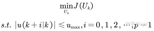
我们从几个角度来解析两者关系，简单的说就是MPC是带了约束的LQR.

在陈虹模型预测控制一书中P20中，提到在目标函数中求得极值的过过程中，相当于对输出量以及状态量相当于加的软约束

而模型预测控制与LQR中其中不同的一点，就是MPC中可以加入硬约束进行对状态量以及输出量的硬性约束

形如：S.T.表示的硬性约束，在LQR中没有这一项

下面我们从代码的角度解析这个问题：
1， 定义被控系统：

1 A = [1.1 2; 0 0.95];
2 B = [0; 0.0787];
3 C = [-1 1];
4 D = 0;
5 Ts = 1;
6 sys = ss(A,B,C,D,Ts);
7 x0 = [0.5;-0.5]; % initial states at [0.5 -0.5]

2，设计无约束LQR：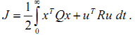

1 Qy = 1;
2 R = 0.01;
3 K_lqr = lqry(sys,Qy,R);

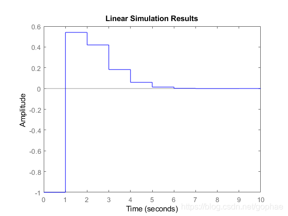
3, 运行仿真闭环结果：

1 t_unconstrained = 0:1:10;
2 u_unconstrained = zeros(size(t_unconstrained));
3 Unconstrained_LQR = tf([-1 1])*feedback(ss(A,B,eye(2),0,Ts),K_lqr);
4 lsim(Unconstrained_LQR,'-',u_unconstrained,t_unconstrained,x0);
5 hold on;

4，设计MPC控制器：

 1 %%
 2 % The MPC objective function is |J(k) = sum(x(k)'*Q*x(k) + u(k)'*R*u(k) +
 3 % x(k+N)'*Q_bar*x(k+N))|. To ensure that the MPC objective function has the
 4 % same quadratic cost as the infinite horizon quadratic cost used by LQR,
 5 % terminal weight |Q_bar| is obtained by solving the following Lyapunov
 6 % equation:
 7 Q = C'*C;
 8 Q_bar = dlyap((A-B*K_lqr)', Q+K_lqr'*R*K_lqr);
 9
10 %%
11 % Convert the MPC problem into a standard QP problem, which has the
12 % objective function |J(k) = U(k)'*H*U(k) + 2*x(k)'*F'*U(k)|.
13 Q_hat = blkdiag(Q,Q,Q,Q_bar);
14 R_hat = blkdiag(R,R,R,R);
15 H = CONV'*Q_hat*CONV + R_hat;
16 F = CONV'*Q_hat*M;
17
18 %%
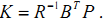
19 % When there are no constraints, the optimal predicted input sequence U(k)
20 % generated by MPC controller is |-K*x|, where |K = inv(H)*F|.
21 K = H\F;
22
23 %%
24 % In practice, only the first control move |u(k) = -K_mpc*x(k)| is applied
25 % to the plant (receding horizon control).
26 K_mpc = K(1,:);
27
28 %%
29 % Run a simulation with initial states at [0.5 -0.5]. The closed-loop
30 % response is stable.
31 Unconstrained_MPC = tf([-1 1])*feedback(ss(A,B,eye(2),0,Ts),K_mpc);
32 lsim(Unconstrained_MPC,'*',u_unconstrained,t_unconstrained,x0)
33 legend show

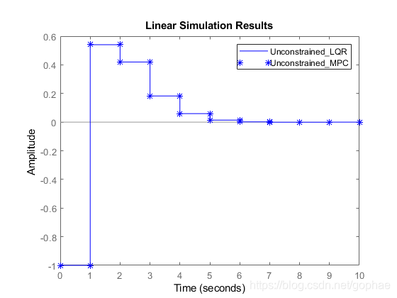
到这里，完全可以说明，在无约束前提下，两种方法是一致的：

1 K_lqr =
2
3     4.3608   18.7401
4
5
6 K_mpc =
7
8     4.3608   18.7401

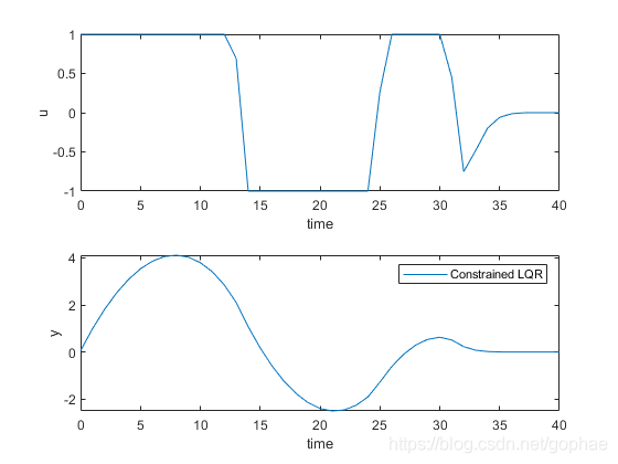
5，对LQR施加约束：

 1 x = x0;
 2 t_constrained = 0:40;
 3 for ct = t_constrained
 4 uLQR(ct+1) = -K_lqrx;
 5 uLQR(ct+1) = max(-1,min(1,uLQR(ct+1)));
 6 x = Ax+BuLQR(ct+1);
 7 yLQR(ct+1) = Cx;
 8 end
 9 figure
10 subplot(2,1,1)
11 plot(t_constrained,uLQR)
12 xlabel(‘time’)
13 ylabel(‘u’)
14 subplot(2,1,2)
15 plot(t_constrained,yLQR)
16 xlabel(‘time’)
17 ylabel(‘y’)
18 legend(‘Constrained LQR’)

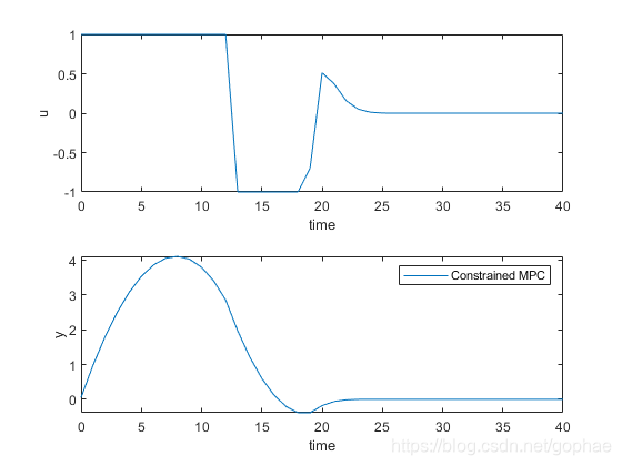
6，对MPC施加约束：

 1 %% MPC Controller Solves QP Problem Online When Applying Constraints
 2 % One of the major benefits of using MPC controller is that it handles
 3 % input and output constraints explicitly by solving an optimization
 4 % problem at each control interval.
 5 %
 6 % Use the built-in KWIK QP solver, |mpcqpsolver|, to implement the custom
 7 % MPC controller designed above. The constraint matrices are defined as
 8 % Ac*x>=b0.
 9 Ac = -[1 0 0 0;...
10       -1 0 0 0;...
11        0 1 0 0;...
12        0 -1 0 0;...
13        0 0 1 0;...
14        0 0 -1 0;...
15        0 0 0 1;...
16        0 0 0 -1];
17 b0 = -[1;1;1;1;1;1;1;1];
18
19 %%
20 % The |mpcqpsolver| function requires the first input to be the inverse of
21 % the lower-triangular Cholesky decomposition of the Hessian matrix H.
22 L = chol(H,'lower');
23 Linv = L\eye(size(H,1));
24
25 %%
26 % Run a simulation by calling |mpcqpsolver| at each simulation step.
27 % Initially all the inequalities are inactive (cold start).
28 x = x0;
29 iA = false(size(b0));
30 opt = mpcqpsolverOptions;
31 opt.IntegrityChecks = false;
32 for ct = t_constrained
33     [u, status, iA] = mpcqpsolver(Linv,F*x,Ac,b0,[],zeros(0,1),iA,opt);
34     uMPC(ct+1) = u(1);
35     x = A*x+B*uMPC(ct+1);
36     yMPC(ct+1) = C*x;
37 end
38 figure
39 subplot(2,1,1)
40 plot(t_constrained,uMPC)
41 xlabel('time')
42 ylabel('u')
43 subplot(2,1,2)
44 plot(t_constrained,yMPC)
45 xlabel('time')
46 ylabel('y')
47 legend('Constrained MPC')

转载：https://blog.csdn.net/gophae/article/details/104546805/