ElasticSearch评分分析 explian 解释和一些查询理解

按照es-ik分析器安装了ik分词器。创建索引：PUT /index_ik_test。索引包含2个字段：content和nick，如下：

GET index_ik_test/_mapping

{

  "index_ik_test": {

    "mappings": {

      "fulltext": {

        "properties": {

          "content": {

            "type": "text",

            "analyzer": "ik_max_word"

          },

          "nick": {

            "type": "text",

            "fields": {

              "keyword": {

                "type": "keyword",

                "ignore_above": 256

              }

            }

          }

        }

      }

    }

  }

}

实验环境为：单台的ElasticSearch6.3.2版本。索引配置如下：

GET index_ik_test/_settings

{

  "index_ik_test": {

    "settings": {

      "index": {

        "creation_date": "1533383757075",

        "number_of_shards": "5",

        "number_of_replicas": "1",

        "uuid": "JajsYmAIT0-uhm-L5xKbeA",

        "version": {

          "created": "6030299"

        },

        "provided_name": "index_ik_test"

      }

    }

  }

}

由此可知，ElasticSearch创建索引时，默认为5个primary shard，每个primary shard 一个replica。

在Kibana的Monitoring界面查看：有5个primary shard。其中有5个尚未分配的副本：

为什么有5个尚未分配的副本呢？因为是单节点的ElasticSearch，索引 index_ik_test 的每个primary shard 都有一个副本，而primary shard 与副本不能在同一台机器上，由于一共有5个primary shard，故存在着5个尚未分配的副本。

该索引一共存储着5篇文档，

GET index_ik_test/fulltext/_search

{

  "query": {

    "match_all": {}

  }

}

查询文档如下：

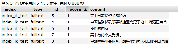
这5篇文档中有三篇文档（文档id为 5、4、3）包含了词 “中国”。由于采用的ik_max_word分词，因此“其中国家投资了500万”，是包含“中国”这个词的。

每个分片中存储的文档如下：

其中，shard2代表分片：[index_ik_test][2] ，shard2上存储着 doc id为 4和6 的两篇文档。shard1 代表分片：[index_ik_test][1]，shard1上存储着文档id为 5 的一篇文档。其它分片存储的文档以此类推。（是不是很奇怪我是怎么知道每个分片上存储具体哪篇文档的？这是因为：在这个演示环境中，文档数量少，我是通过不同的查询词（比如通过 query explian "我们"，就能知道 doc_6 存储在shard2上了）进行explian查询测试得到的。哈哈，知道这个主要是为了后面的 idf 计算分析）

下面以词 "中国" 为例来解释：query explian。执行：

GET index_ik_test/fulltext/_search

{

  "explain": true,

  "query": {

    "match": {

      "content": "中国"

    }

  }

}

下面从该命令的执行结果详细分析：

{

"took": 1,

"timed_out": false,

"_shards": {

"total": 5,

"successful": 5,

"skipped": 0,

"failed": 0

},

"hits": {

"total": 3,

"max_score": 0.5480699,

这表明，查询请求 scatter 到了所有的 shard （5个shard），其中有3个shard “命中了” 查询词 “中国”。这3个shard如下：

"_shard": "[index_ik_test][2]"

"_shard": "[index_ik_test][1]"

"_shard": "[index_ik_test][4]"

每个shard都会计算一个score，这3个shard中，得分最大的分片是shard2 [index_ik_test][2]，它的score是：0.5480699。因此，shard2上的返回结果排在了最前面，只是这里有个小疑问，为什么score返回结果是取最大值(max_score)？

对于 shard`[index_ik_test][2]`：

    "_shard": "[index_ik_test][2]",

    "_node": "7MyDkEDrRj2RPHCPoaWveQ",

    "_index": "index_ik_test",

    "_type": "fulltext",

    "_id": "4",

    "_score": 0.5480699,

    "_source": {

      "content": "中国驻洛杉矶领事馆遭亚裔男子枪击 嫌犯已自首"

    },

文档id 4 存储在shard2 上。该文档针对查询字符串 “中国” 计算出来的得分是0.5480699。具体的计算细节如下：

   "_explanation": {

          "value": 0.5480699,

          "description": "weight(content:中国 in 0) [PerFieldSimilarity], result of:",

          "details": [

            {

              "value": 0.5480699,

              "description": "score(doc=0,freq=1.0 = termFreq=1.0\n), product of:",

              "details": [

                {

                  "value": 0.6931472,

                  "description": "idf, computed as log(1 + (docCount - docFreq + 0.5) / (docFreq + 0.5)) from:",

                  "details": [

                    {

                      "value": 1,

                      "description": "docFreq",

                      "details": []

                    },

                    {

                      "value": 2,

                      "description": "docCount",

                      "details": []

                    }

                  ]

                },

                {

                  "value": 0.7906977,

                  "description": "tfNorm, computed as (freq * (k1 + 1)) / (freq + k1 * (1 - b + b * fieldLength / avgFieldLength)) from:",

                  "details": [

                    {

                      "value": 1,

                      "description": "termFreq=1.0",

                      "details": []

                    },

                    {

                      "value": 1.2,

                      "description": "parameter k1",

                      "details": []

                    },

                    {

                      "value": 0.75,

                      "description": "parameter b",

                      "details": []

                    },

                    {

                      "value": 8.5,

                      "description": "avgFieldLength",

                      "details": []

                    },

                    {

                      "value": 14,

                      "description": "fieldLength",

                      "details": []

                    }

                  ]

                }

              ]

            }

          ]

        }

0.5480699 由idf 乘以 tfNorm 计算得到。其中 idf=0.6931472，tfNorm=0.7906977

idf

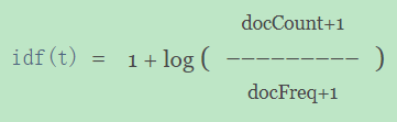
idf由公式 log(1 + (docCount - docFreq + 0.5) / (docFreq + 0.5))计算得出。其中，docFreq=1，docCount=2，因为如上面图所示：在shard2上，一共有2篇文档，因此docCount为2，其中只有文档id为4的这篇文档包含 "中国" 这个词，也即：词 "中国" 出现在了一篇文档中，因此docFreq=1。

不信的话就亲自动手算算看。^~

我这里有疑问的地方是：这里的 idf 计算公式与官网提到的计算公式有一点不一样：

后来发现，在ElasticSearch6.3版本之后，字段评分算法默认是BM25算法了。

Elasticsearch allows you to configure a scoring algorithm or similarity per field. The similarity setting provides a simple way of choosing a similarity algorithm other than the default BM25, such as TF/IDF.

在BM25算法的官方文档API中发现IDF的计算公式如下：

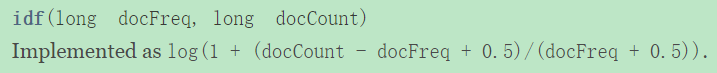
这样也就知道了，ElasticSearch在计算Term的字段得分是，采用的是BM25算法。计算出该term在这个字段中的idf值后，再结合其他因子（比如tf、字段长度Normalization、文档长度Normalization）最终得出文档的Score。

那么tf-idf与BM25的区别是什么？tf-idf是一个term scoring method，而BM25是：给定一个查询字符串，计算该查询字符串与文档之间的得分的一种方法。文档是由一个个的term组成的，计算文档得分需要计算文档中term的得分。将tf-idf结合余弦相似度就是另外一种计算查询字符串与文档之间的得分的一种方法。

BM25 is more than a term scoring method, but rather a method for scoring documents with relation to a query. Tf-idf is a term scoring method, which can be incorporated in a document scoring method using a similarity measure (say cosine).

并且BM25的理论基础是probabilistic retrieval model，而tf-idf的理论基础是 vector space model。

docFreq=1表示："中国"这个词只在一篇文档中出现了。

https://lucene.apache.org/core/7_4_0/core/org/apache/lucene/search/similarities/TFIDFSimilarity.html

docFreq (the number of documents in which the term t appears)

docFreq - the number of documents which contain the term

docCount - the total number of documents in the collection

dcoCount=2表示：分片[index_ik_test][2] 里面一共存储了2篇文档(即doc_4 和 doc_6)。

tfNorm

tfNorm由公式(freq * (k1 + 1)) / (freq + k1 * (1 - b + b * fieldLength / avgFieldLength))计算。
1. freq ，即termFreq，应该是：term 在该分片下的所有文档中出现的频率。在这里，“中国” 在 shard2 的两篇文档中，只出现过一次
2. k1 ，这个参数很有意思，默认值为1.2，是用来平衡词频termFreq 对评分的影响。在传统的TF评分计算过程中，termFreq越大，计算出来的评分就越大。但是当termFreq大到一定程度时，一般是那种常用词(或者叫stop words)，而这种词会干扰文档的评分，因此引入参数 k1 惩罚 termFreq 对评分的影响。要想了解更多，可参考这篇文章：bm25-the-next-generation-of-lucene-relevation。这里也说明，ElasticSearch6.3.2中已经采用了BM25算法作为相关性得分计算公式了。
  
  https://www.desmos.com/calculator/g8zoebbtvs
3. b，从tfNorm公式可看出：用来调节字段长度对评分的影响。
4. avgFieldLength 值为8.5。为什么是8.5呢？
  
  在我们的示例中，shard2 [index_ik_test][2]中一共存储了2篇文档，一篇是doc_4，它的content字段就是"中国驻洛杉矶领事馆遭亚裔男子枪击嫌犯已自首"。另一篇是doc_6，它的content字段是"我们的国家"。
  
  对doc_6的content字段进行分析：
```
GET index_ik_test/_analyze

{

  "text": ["我们的国家"],

  "analyzer": "ik_max_word"

}

得到的各个 token 如下：

我们、的、国家

一共3个token
```
  在下面的第五点fieldLength中，对doc_4的content字段进行分析得到 14个token。
  
  因此，avgFieldLength = （14+3）/2=8.5。14 是doc_4 content字段分词之后的token数目；3是doc_6 content字段分词之后的token数目；2 代表：有两篇文档。
  
  由此可知：avgFieldLength 应该是：shard2分片中 content字段下所有内容经过 ik_max_word 分词后的token 总数除以 shard2里面的文档数目。
5. fieldLength，长度为14。这个是doc_4 “中国驻洛杉矶领事馆遭亚裔男子枪击嫌犯已自首” ik_max_word分词之后的长度。因此，fieldLength指的是查询字段(content字段) 被分析(创建索引时指定了 ik_max_word分析器) 之后的长度。
```
GET index_ik_test/_analyze

{

  "text": ["中国驻洛杉矶领事馆遭亚裔男子枪击 嫌犯已自首"],

  "analyzer": "ik_max_word"

}

得到的各个token如下：

中国、驻、洛杉矶、领事馆、领事、馆、遭、亚裔、男子、子枪、枪击、嫌犯、已、自首

一共 14 个token
```
  各个参数的值以及计算过程如下：
freq=1.0

k1=1.2

b=0.75

avgFieldLength=8.5

fieldLength=14

(freq*(k1+1))/(freq+k1*(1-b+b*fieldLength/avgFieldLength))

0.7906976744186047

现在，针对shard2，我们已经详细分析了 tfNorm 和 idf 这两个参数的计算结果。最终，shard2上的查询得分为 tfNorm*idf=0.7906977*0.6931472=0.5480699 。另外两个命中 “中国” 的分片的得分计算也类似，就不说了。

由此可看出：ElasticSearch中 tf-idf 的值是根据单个分片来计算的，也即：以单个的shard为单位来计算 score，更具体地说：当我们讲某 term 一共在文档集合中出现了多少次？这个文档集合指的是：单个分片上存储的所有文档。为什么是统计单个分片上的文档/term 数量呢？这个就要从ElasticSearch的索引方式说起了。这里就简单地提一下，毕竟这不是本文的重点。

ElasticSearch中有两个不同Level的索引，一个是：文档到分片这个级别的索引，它讲的是数据的分布方式，即决定把哪篇文档存储在哪个分片上，这是通过hash文档ID的方式来实现的。采用hash方式的好处是，ElasticSearch不需要维护文档的位置信息(boundary)，文档能够均匀地分布在各个shard上。ElasticSearch采用的哈希函数是：murmur3。

另一个级别的索引是：term 到文档的索引，俗称倒排索引，又称为：Secondary index。因为我们的查询需求并不是：给定一个docId，返回这个docId所代表的文档内容。我们的查询需求是：给定一个查询关键词，找出哪些docId 包含了这个查询关键词。因此，要完成这个查询，第一步是要知道有哪些docId 包含了查询关键词；第二步则是：根据docId，拿到相应的文档内容。

当文档的数量很多很多时，一台机器或者说一个shard都存储不下这个倒排索引了，因此需要对倒排索引进行分割(partition)。一种分割方式是：Secondary index by Document，另一种是：Secondary index by Term。

Secondary index by Document的示意图如下：（这里的Partition 可以与 ElasticSearch中的 shard 概念等价）

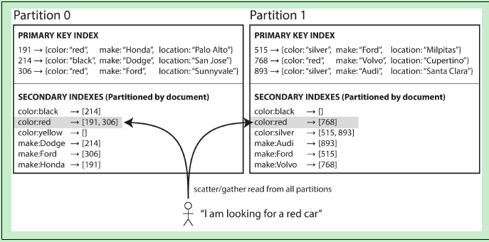
这种Secondary Index的分布方式（或者叫数据分布方式，这里的数据当然是倒排索引数据了）是针对每个Partition上的文档建立一个独立的Secondary Index(倒排索引)。这种索引方式的好处是：当写入/更新文档时，只涉及到该Partition中的倒排索引，而不会修改其他的Partition中的倒排索引内容。

更具体地，以ElasticSearch举例，因为ElasticSearch就是采用Secondary index by Document。当创建索引时，是默认5个Primary shard，每个Primary shard 一个副本(replica)。Primary shard 就相当于这里的Partition概念。当向ElasticSearch的索引中写入文档时，写请求是请求给某个Primary shard，然后在该Primary shard上构建倒排索引(posting list)，而并不需要修改其他4个Primary shard 中的倒排索引内容。

each partition is completely separate: each partition maintains its own secondary indexes, covering only the documents in that partition. It doesn’t care what data is stored in other partitions.

因此，查询的时候，需要将查询请求发送到每一个partition(shard)。为什么呢？因为当我们查询的时候，一般是输入某个词进行查询，比如输入"中国"进行查询，而由于Elasticsearch采用 secondary index by document 这种方式，各个shard 维护着自己的 secondary index，比如，在文档1 中包含了 "中国" 这个词，而文档1 被哈希分片到 shard1中存储；文档2也包含了"中国" 这个词，但是文档2可能被哈希到另外一个shard，比如shard2上存储……因此，所有包含"中国" 这个词的文档可能分布在 Elasticsearch的所有分片中，因此查询请求需要分发到每个shard上去，这就是所谓的Scatter 查询。当然了，由于primary shard可以设置若干个 replica，因此，将查询请求分发到 replica上，通过 replica 来扛大量的查询请求。毕竟 index操作(将文档写入Elasticsearch)是由primary shard处理的，那将查询请求交由 replica处理，一定程度上缓解了primary shard的压力。

Secondary index by Term示意图如下：

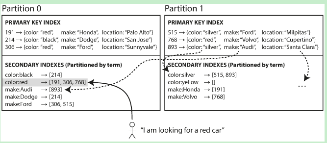
这种Secondary index的分布方式是按”范围“ 来进行分布，关于数据的分布方式，可参考：[分布式系统原理介绍。比如说，对于 color 这个字段，颜色有 black、red、silver……文档中颜色范围首字母为 [a-r] 的那些docId 存储在 Partition0 分片上。而所有颜色范围首字母 [s-z] 的docId，则存储在Partition1分片上。采用这种分布方式的倒排索引，一篇文档中的不同字段可能会在多个Partition的字段中被索引。比如，文档893 的color 字段的内容是 silver，它在Partition1中被索引了；而文档893的make字段内容是Audi，它在Partition0中被索引了。这种索引方式的缺点显而易见：当更新/插入一篇文档时，有可能需要更新多个Partition中的倒排索引内容。因此，查询的时候，可以只将查询请求发送到某个特定的partition(shard)。

以上内容，全是自己的理解。可能会有很多不严谨的地方。

补充说明

这篇文章记录的文档得分计算比较简单：1，它只涉及到单个字段查询，即只查询content字段；2，查询字符串只有一个term，即：“中国”。

而现实中的查询，查询字符串可能包含多个term，并且针对索引中的多个字段查询。因此，文档得分的计算要复杂得多。

参考文献：

最后，放一份完整的explian 查询分析返回内容：

{
"took": 1,
"timed_out": false,
"_shards": {
"total": 5,
"successful": 5,
"skipped": 0,
"failed": 0
},
"hits": {
"total": 3,
"max_score": 0.5480699,
"hits": [
{
"_shard": "[index_ik_test][2]",
"_node": "7MyDkEDrRj2RPHCPoaWveQ",
"_index": "index_ik_test",
"_type": "fulltext",
"_id": "4",
"_score": 0.5480699,
"_source": {
"content": "中国驻洛杉矶领事馆遭亚裔男子枪击嫌犯已自首"
},
"_explanation": {
"value": 0.5480699,
"description": "weight(content:中国 in 0) [PerFieldSimilarity], result of:",
"details": [
{
"value": 0.5480699,
"description": "score(doc=0,freq=1.0 = termFreq=1.0\n), product of:",
"details": [
{
"value": 0.6931472,
"description": "idf, computed as log(1 + (docCount - docFreq + 0.5) / (docFreq + 0.5)) from:",
"details": [
{
"value": 1,
"description": "docFreq",
"details": []
},
{
"value": 2,
"description": "docCount",
"details": []
}
]
},
{
"value": 0.7906977,
"description": "tfNorm, computed as (freq * (k1 + 1)) / (freq + k1 * (1 - b + b * fieldLength / avgFieldLength)) from:",
"details": [
{
"value": 1,
"description": "termFreq=1.0",
"details": []
},
{
"value": 1.2,
"description": "parameter k1",
"details": []
},
{
"value": 0.75,
"description": "parameter b",
"details": []
},
{
"value": 8.5,
"description": "avgFieldLength",
"details": []
},
{
"value": 14,
"description": "fieldLength",
"details": []
}
]
}
]
}
]
}
},
{
"_shard": "[index_ik_test][1]",
"_node": "7MyDkEDrRj2RPHCPoaWveQ",
"_index": "index_ik_test",
"_type": "fulltext",
"_id": "5",
"_score": 0.2876821,
"_source": {
"content": "其中国家投资了500万"
},
"_explanation": {
"value": 0.2876821,
"description": "weight(content:中国 in 0) [PerFieldSimilarity], result of:",
"details": [
{
"value": 0.2876821,
"description": "score(doc=0,freq=1.0 = termFreq=1.0\n), product of:",
"details": [
{
"value": 0.2876821,
"description": "idf, computed as log(1 + (docCount - docFreq + 0.5) / (docFreq + 0.5)) from:",
"details": [
{
"value": 1,
"description": "docFreq",
"details": []
},
{
"value": 1,
"description": "docCount",
"details": []
}
]
},
{
"value": 1,
"description": "tfNorm, computed as (freq * (k1 + 1)) / (freq + k1 * (1 - b + b * fieldLength / avgFieldLength)) from:",
"details": [
{
"value": 1,
"description": "termFreq=1.0",
"details": []
},
{
"value": 1.2,
"description": "parameter k1",
"details": []
},
{
"value": 0.75,
"description": "parameter b",
"details": []
},
{
"value": 7,
"description": "avgFieldLength",
"details": []
},
{
"value": 7,
"description": "fieldLength",
"details": []
}
]
}
]
}
]
}
},
{
"_shard": "[index_ik_test][4]",
"_node": "7MyDkEDrRj2RPHCPoaWveQ",
"_index": "index_ik_test",
"_type": "fulltext",
"_id": "3",
"_score": 0.2876821,
"_source": {
"content": "中韩渔警冲突调查：韩警平均每天扣1艘中国渔船"
},
"_explanation": {
"value": 0.2876821,
"description": "weight(content:中国 in 0) [PerFieldSimilarity], result of:",
"details": [
{
"value": 0.2876821,
"description": "score(doc=0,freq=1.0 = termFreq=1.0\n), product of:",
"details": [
{
"value": 0.2876821,
"description": "idf, computed as log(1 + (docCount - docFreq + 0.5) / (docFreq + 0.5)) from:",
"details": [
{
"value": 1,
"description": "docFreq",
"details": []
},
{
"value": 1,
"description": "docCount",
"details": []
}
]
},
{
"value": 1,
"description": "tfNorm, computed as (freq * (k1 + 1)) / (freq + k1 * (1 - b + b * fieldLength / avgFieldLength)) from:",
"details": [
{
"value": 1,
"description": "termFreq=1.0",
"details": []
},
{
"value": 1.2,
"description": "parameter k1",
"details": []
},
{
"value": 0.75,
"description": "parameter b",
"details": []
},
{
"value": 14,
"description": "avgFieldLength",
"details": []
},
{
"value": 14,
"description": "fieldLength",
"details": []
}
]
}
]
}
]
}
}
]
}
}

原文：https://www.cnblogs.com/hapjin/p/9677753.html