Holm–Bonferroni method

python机器学习-乳腺癌细胞挖掘（博主亲自录制视频）https://study.163.com/course/introduction.htm?courseId=1005269003&utm_campaign=commission&utm_source=cp-400000000398149&utm_medium=share

项目合作：QQ231469242

# -*- coding: utf-8 -*-

# Import standard packages

import numpy as np

from scipy import stats

import pandas as pd

import os

# Other required packages

from statsmodels.stats.multicomp import (pairwise_tukeyhsd,

                                         MultiComparison)

from statsmodels.formula.api import ols

from statsmodels.stats.anova import anova_lm

#数据excel名

excel="sample.xlsx"

#读取数据

df=pd.read_excel(excel)

#获取第一组数据，结构为列表

group_mental=list(df.StressReduction[(df.Treatment=="mental")])

group_physical=list(df.StressReduction[(df.Treatment=="physical")])

group_medical=list(df.StressReduction[(df.Treatment=="medical")])

multiComp = MultiComparison(df['StressReduction'], df['Treatment'])

def Holm_Bonferroni(multiComp):

    ''' Instead of the Tukey's test, we can do pairwise t-test

    通过均分a=0.05,矫正a,得到更小a'''

    # First, with the "Holm" correction

    rtp = multiComp.allpairtest(stats.ttest_rel, method='Holm')

    print((rtp[0]))

    # and then with the Bonferroni correction

    print((multiComp.allpairtest(stats.ttest_rel, method='b')[0]))

    # Any value, for testing the program for correct execution

    checkVal = rtp[1][0][0,0]

    return checkVal

Holm_Bonferroni(multiComp)

数据sample.xlsx

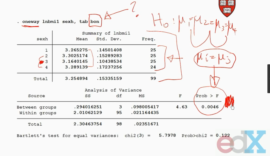
因为反复比较，一型错误概率会增加。

bonferroni 矫正一型错误的公式，它减少了a=0.05关键值

例如有5组数比较，比较的配对结果有10个

所以矫正的a=0.05/10=0.005

https://en.wikipedia.org/wiki/Holm%E2%80%93Bonferroni_method

In statistics, the Holm–Bonferroni method^[1] (also called the Holm method or Bonferroni-Holm method) is used to counteract the problem of multiple comparisons. It is intended to control the familywise error rate and offers a simple test uniformly more powerful than the Bonferroni correction. It is one of the earliest usages of stepwise algorithms in simultaneous inference. It is named after Sture Holm, who codified the method, and Carlo Emilio Bonferroni.

Motivation

When considering several hypotheses, the problem of multiplicity arises: the more hypotheses we check, the higher the probability of a Type I error (false positive). The Holm–Bonferroni method is one of many approaches that control the family-wise error rate (the probability that one or more Type I errors will occur) by adjusting the rejection criteria of each of the individual hypotheses or comparisons.

Formulation

The method is as follows:

Let H 1 , . . . , H m {\displaystyle H_{1},...,H_{m}} be a family of hypotheses and P 1 , . . . , P m {\displaystyle P_{1},...,P_{m}} the corresponding P-values.
Start by ordering the p-values (from lowest to highest) P ( 1 ) … P ( m ) {\displaystyle P_{(1)}\ldots P_{(m)}} and let the associated hypotheses be H ( 1 ) … H ( m ) {\displaystyle H_{(1)}\ldots H_{(m)}}
For a given significance level α {\displaystyle \alpha } , let k {\displaystyle k} be the minimal index such that P ( k ) > α m + 1 − k {\displaystyle P_{(k)}>{\frac {\alpha }{m+1-k}}}
Reject the null hypotheses H ( 1 ) … H ( k − 1 ) {\displaystyle H_{(1)}\ldots H_{(k-1)}} and do not reject H ( k ) … H ( m ) {\displaystyle H_{(k)}\ldots H_{(m)}}
If k = 1 {\displaystyle k=1} then do not reject any of the null hypotheses and if no such k {\displaystyle k} exist then reject all of the null hypotheses.

The Holm–Bonferroni method ensures that this method will control the F W E R ≤ α {\displaystyle FWER\leq \alpha } , where F W E R {\displaystyle FWER} is the familywise error rate

Proof

Holm-Bonferroni controls the FWER as follows. Let H ( 1 ) … H ( m ) {\displaystyle H_{(1)}\ldots H_{(m)}} be a family of hypotheses, and P ( 1 ) ≤ P ( 2 ) ≤ … ≤ P ( m ) {\displaystyle P_{(1)}\leq P_{(2)}\leq \ldots \leq P_{(m)}} be the sorted p-values. Let I 0 {\displaystyle I_{0}} be the set of indices corresponding to the (unknown) true null hypotheses, having m 0 {\displaystyle m_{0}} members.

Let us assume that we wrongly reject a true hypothesis. We have to prove that the probability of this event is at most α {\displaystyle \alpha } . Let h {\displaystyle h} be the first rejected true hypothesis (first in the ordering given by the Bonferroni–Holm test). So h − 1 {\displaystyle h-1} is the last false hypothesis rejected and h − 1 + m 0 ≤ m {\displaystyle h-1+m_{0}\leq m} . From there, we get 1 m − h + 1 ≤ 1 m 0 {\displaystyle {\frac {1}{m-h+1}}\leq {\frac {1}{m_{0}}}} (1). Since h {\displaystyle h} is rejected we have P ( h ) ≤ α m + 1 − h {\displaystyle P_{(h)}\leq {\frac {\alpha }{m+1-h}}} by definition of the test. Using (1), the right hand side is at most α m 0 {\displaystyle {\frac {\alpha }{m_{0}}}} . Thus, if we wrongly reject a true hypothesis, there has to be a true hypothesis with P-value at most α m 0 {\displaystyle {\frac {\alpha }{m_{0}}}} .

So let us define A = { P i ≤ α m 0 for some i ∈ I 0 } {\displaystyle A=\left\{P_{i}\leq {\frac {\alpha }{m_{0}}}{\text{ for some }}i\in I_{0}\right\}} . Whatever the (unknown) set of true hypotheses I 0 {\displaystyle I_{0}} is, we have Pr ( A ) ≤ α {\displaystyle \Pr(A)\leq \alpha } (by the Bonferroni inequalities). Therefore, the probability to reject a true hypothesis is at most α {\displaystyle \alpha } .

Alternative proof

The Holm–Bonferroni method can be viewed as closed testing procedure,^[2] with Bonferroni method applied locally on each of the intersections of null hypotheses. As such, it controls the familywise error rate for all the k hypotheses at level α in the strong sense. Each intersection is tested using the simple Bonferroni test.

It is a shortcut procedure since practically the number of comparisons to be made equal to m {\displaystyle m} or less, while the number of all intersections of null hypotheses to be tested is of order 2 m {\displaystyle 2^{m}} .

The closure principle states that a hypothesis H i {\displaystyle H_{i}} in a family of hypotheses H 1 , . . . , H m {\displaystyle H_{1},...,H_{m}} is rejected - while controlling the family-wise error rate of α {\displaystyle \alpha } - if and only if all the sub-families of the intersections with H i {\displaystyle H_{i}} are controlled at level of family-wise error rate of α {\displaystyle \alpha } .

In Holm-Bonferroni procedure, we first test H ( 1 ) {\displaystyle H_{(1)}} . If it is not rejected then the intersection of all null hypotheses ⋂ i = 1 m H i {\displaystyle \bigcap \nolimits _{i=1}^{m}{H_{i}}} is not rejected too, such that there exist at least one intersection hypothesis for each of elementary hypotheses H 1 , . . . , H m {\displaystyle H_{1},...,H_{m}} that is not rejected, thus we reject none of the elementary hypotheses.

If H ( 1 ) {\displaystyle H_{(1)}} is rejected at level α / m {\displaystyle \alpha /m} then all the intersection sub-families that contain it are rejected too, thus H ( 1 ) {\displaystyle H_{(1)}} is rejected. This is because P ( 1 ) {\displaystyle P_{(1)}} is the smallest in each one of the intersection sub-families and the size of the sub-families is the most m {\displaystyle m} , such that the Bonferroni threshold larger than α / m {\displaystyle \alpha /m} .

The same rationale applies for H ( 2 ) {\displaystyle H_{(2)}} . However, since H ( 1 ) {\displaystyle H_{(1)}} already rejected, it sufficient to reject all the intersection sub-families of H ( 2 ) {\displaystyle H_{(2)}} without H ( 1 ) {\displaystyle H_{(1)}} . Once P ( 2 ) ≤ α / ( m − 1 ) {\displaystyle P_{(2)}\leq \alpha /(m-1)} holds all the intersections that contains H ( 2 ) {\displaystyle H_{(2)}} are rejected.

The same applies for each 1 ≤ i ≤ m {\displaystyle 1\leq i\leq m} .

Example

Consider four null hypotheses H 1 , . . . , H 4 {\displaystyle H_{1},...,H_{4}} with unadjusted p-values p 1 = 0.01 {\displaystyle p_{1}=0.01} , p 2 = 0.04 {\displaystyle p_{2}=0.04} , p 3 = 0.03 {\displaystyle p_{3}=0.03} and p 4 = 0.005 {\displaystyle p_{4}=0.005} , to be tested at significance level α = 0.05 {\displaystyle \alpha =0.05} . Since the procedure is step-down, we first test H 4 = H ( 1 ) {\displaystyle H_{4}=H_{(1)}} , which has the smallest p-value p 4 = p ( 1 ) = 0.005 {\displaystyle p_{4}=p_{(1)}=0.005} . The p-value is compared to α / 4 = 0.0125 {\displaystyle \alpha /4=0.0125} , the null hypothesis is rejected and we continue to the next one. Since p 1 = p ( 2 ) = 0.01 < 0.0167 = α / 3 {\displaystyle p_{1}=p_{(2)}=0.01<0.0167=\alpha /3} we reject H 1 = H ( 2 ) {\displaystyle H_{1}=H_{(2)}} as well and continue. The next hypothesis H 3 {\displaystyle H_{3}} is not rejected since p 3 = p ( 3 ) = 0.03 > 0.025 = α / 2 {\displaystyle p_{3}=p_{(3)}=0.03>0.025=\alpha /2} . We stop testing and conclude that H 1 {\displaystyle H_{1}} and H 4 {\displaystyle H_{4}} are rejected and H 2 {\displaystyle H_{2}} and H 3 {\displaystyle H_{3}} are not rejected while controlling the familywise error rate at level α = 0.05 {\displaystyle \alpha =0.05} . Note that even though p 2 = p ( 4 ) = 0.04 < 0.05 = α {\displaystyle p_{2}=p_{(4)}=0.04<0.05=\alpha } applies, H 2 {\displaystyle H_{2}} is not rejected. This is because the testing procedure stops once a failure to reject occurs.

Extensions

Holm–Šidák method

Further information: Šidák correction

When the hypothesis tests are not negatively dependent, it is possible to replace α m , α m − 1 , . . . , α 1 {\displaystyle {\frac {\alpha }{m}},{\frac {\alpha }{m-1}},...,{\frac {\alpha }{1}}} with:

1 − ( 1 − α ) 1 / m , 1 − ( 1 − α ) 1 / ( m − 1 ) , . . . , 1 − ( 1 − α ) 1 {\displaystyle 1-(1-\alpha )^{1/m},1-(1-\alpha )^{1/(m-1)},...,1-(1-\alpha )^{1}}

resulting in a slightly more powerful test.

Weighted version

Let P ( 1 ) , . . . , P ( m ) {\displaystyle P_{(1)},...,P_{(m)}} be the ordered unadjusted p-values. Let H ( i ) {\displaystyle H_{(i)}} , 0 ≤ w ( i ) {\displaystyle 0\leq w_{(i)}} correspond to P ( i ) {\displaystyle P_{(i)}} . Reject H ( i ) {\displaystyle H_{(i)}} as long as

P ( j ) ≤ w ( j ) ∑ k = j m w ( k ) α , j = 1 , . . . , i {\displaystyle P_{(j)}\leq {\frac {w_{(j)}}{\sum _{k=j}^{m}{w_{(k)}}}}\alpha ,\quad j=1,...,i}

Adjusted p-values

The adjusted p-values for Holm–Bonferroni method are:

p ~ ( i ) = max j ≤ i { ( m − j + 1 ) p ( j ) } 1 {\displaystyle {\widetilde {p}}_{(i)}=\max _{j\leq i}\left\{(m-j+1)p_{(j)}\right\}_{1}}

, where { x } 1 ≡ min ( x , 1 ) {\displaystyle \{x\}_{1}\equiv \min(x,1)}

In the earlier example, the adjusted p-values are p ~ 1 = 0.03 {\displaystyle {\widetilde {p}}_{1}=0.03} , p ~ 2 = 0.06 {\displaystyle {\widetilde {p}}_{2}=0.06} , p ~ 3 = 0.06 {\displaystyle {\widetilde {p}}_{3}=0.06} and p ~ 4 = 0.02 {\displaystyle {\widetilde {p}}_{4}=0.02} . Only hypotheses H 1 {\displaystyle H_{1}} and H 4 {\displaystyle H_{4}} are rejected at level α = 0.05 {\displaystyle \alpha =0.05} .

The weighted adjusted p-values are:^{[citation needed]}

p ~ ( i ) = max j ≤ i { ∑ k = j m w ( k ) w ( j ) p ( j ) } 1 {\displaystyle {\widetilde {p}}_{(i)}=\max _{j\leq i}\left\{{\frac {\sum _{k=j}^{m}{w_{(k)}}}{w_{(j)}}}p_{(j)}\right\}_{1}}

, where { x } 1 ≡ min ( x , 1 ) {\displaystyle \{x\}_{1}\equiv \min(x,1)}

A hypothesis is rejected at level α if and only if its adjusted p-value is less than α. In the earlier example using equal weights, the adjusted p-values are 0.03, 0.06, 0.06, and 0.02. This is another way to see that using α = 0.05, only hypotheses one and four are rejected by this procedure.

Alternatives and usage

Main article: Familywise error rate § Controlling procedures

The Holm–Bonferroni method is uniformly more powerful than the classic Bonferroni correction. There are other methods for controlling the family-wise error rate that are more powerful than Holm-Bonferroni.

In the Hochberg procedure, rejection of H ( 1 ) … H ( k ) {\displaystyle H_{(1)}\ldots H_{(k)}} is made after finding the maximal index k {\displaystyle k} such that P ( k ) ≤ α m + 1 − k {\displaystyle P_{(k)}\leq {\frac {\alpha }{m+1-k}}} . Thus, The Hochberg procedure is more powerful by construction. However, the Hochberg procedure requires the hypotheses to be independent or under certain forms of positive dependence, whereas Holm-Bonferroni can be applied without such assumptions.

A similar step-up procedure is the Hommel procedure.^[3]

Naming

Carlo Emilio Bonferroni did not take part in inventing the method described here. Holm originally called the method the "sequentially rejective Bonferroni test", and it became known as Holm-Bonferroni only after some time. Holm's motives for naming his method after Bonferroni are explained in the original paper: "The use of the Boole inequality within multiple inference theory is usually called the Bonferroni technique, and for this reason we will call our test the sequentially rejective Bonferroni test."

Bonferroni校正：如果在同一数据集上同时检验n个独立的假设，那么用于每一假设的统计显著水平，应为仅检验一个假设时的显著水平的1/n。

简介

编辑

举个例子：如要在同一数据集上检验两个独立的假设，显著水平设为常见的0.05。此时用于检验该两个假设应使用更严格的0.025。即0.05* (1/2)。该方法是由Carlo Emilio Bonferroni发展的，因此称Bonferroni校正。

这样做的理由是基于这样一个事实：在同一数据集上进行多个假设的检验，每20个假设中就有一个可能纯粹由于概率，而达到0.05的显著水平。

维基百科原文

编辑

Bonferroni correction

Bonferroni correction states that if an experimenter is testing n independent hypotheses on a set of data, then the statistical significance level that should be used for each hypothesis separately is 1/n times what it would be if only one hypothesis were tested.

For example, to test two independent hypotheses on the same data at 0.05 significance level, instead of using a p value threshold of 0.05, one would use a stricter threshold of 0.025.

The Bonferroni correction is a safeguard against multiple tests of statistical significance on the same data, where 1 out of every 20 hypothesis-tests will appear to be significant at the α = 0.05 level purely due to chance. It was developed by Carlo Emilio Bonferroni.

A less restrictive criterion is the rough false discovery rate giving (3/4)0.05 = 0.0375 for n = 2 and (21/40)0.05 = 0.02625 for n = 20.

数据分析中常碰见多重检验问题(multiple testing).Benjamini于1995年提出一种方法，是假阳性的.在统计学上，这也就等价于控制FDR不能超过5%.

根据Benjamini在他的文章中所证明的定理，控制fdr的步骤实际上非常简单。

设总共有m个候选基因，每个基因对应的p值从小到大排列分别是p(1),p(2),...,p(m),

The False Discovery Rate (FDR) of a set of predictions is the expected percent of false predictions in the set of predictions. For example if the algorithm returns 100 genes with a false discovery rate of .3 then we should expect 70 of them to be correct.

The FDR is very different from ap-value, and as such a much higher FDR can be tolerated than with a p-value. In the example above a set of 100 predictions of which 70 are correct might be very useful, especially if there are thousands of genes on the array most of which are not differentially expressed. In contrast p-value of .3 is generally unacceptabe in any circumstance. Meanwhile an FDR of as high as .5 or even higher might be quite meaningful.

FDR错误控制法是Benjamini于1995年提出一种方法,通过控制FDR(False Discovery Rate)来决定P值的域值. 假设你挑选了R个差异表达的基因，其中有S个是真正有差异表达的，另外有V个其实是没有差异表达的，是假阳性的。实践中希望错误比例Q=V/R平均而言不能超过某个预先设定的值（比如0.05），在统计学上，这也就等价于控制FDR不能超过5%.

对所有候选基因的p值进行从小到大排序，则若想控制fdr不能超过q，则只需找到最大的正整数i，使得 p(i)<= (i*q)/m.然后，挑选对应p(1),p(2),...,p(i)的基因做为差异表达基因，这样就能从统计学上保证fdr不超过q。因此，FDR的计算公式如下：

p-value(i)=p(i)*length(p)/rank(p)

参考文献

编辑

1.Audic, S. and J. M. Claverie (1997). The significance of digital gene expression profiles. Genome Res 7(10): 986-95.

2.Benjamini, Y. and D. Yekutieli (2001). The control of the false discovery rate in multiple testing under dependency. The Annals of Statistics. 29: 1165-1188.

计算方法请参考 R统计软件的p.adjust函数：

> p<-c(0.0003,0.0001,0.02)

> p

[1] 3e-04 1e-04 2e-02

> p.adjust(p,method="fdr",length(p))

[1] 0.00045 0.00030 0.02000

> p*length(p)/rank(p)

[1] 0.00045 0.00030 0.02000

> length(p)

[1] 3

> rank(p)

[1] 2 1 3

sort(p)

[1] 1e-04 3e-04 2e-02^[1]

参考资料

https://study.163.com/provider/400000000398149/index.htm?share=2&shareId=400000000398149（欢迎关注博主主页，学习python视频资源，还有大量免费python经典文章）