Visualizing LSTM Layer with t-sne in Neural Networks

LSTM 可视化

Visualizing Layer Representations in Neural Networks

Visualizing and interpreting representations learned by machine learning / deep learning algorithms is pretty interesting! As the saying goes — “A picture is worth a thousand words”, the same holds true with visualizations. A lot can be interpreted using the correct tools for visualization. In this post, I will cover some details on visualizing intermediate (hidden) layer features using dimension reduction techniques.

We will work with the IMDB sentiment classification task (25000 training and 25000 test examples). The script to create a simple Bidirectional LSTM model using a dropout and predicting the sentiment (1 for positive and 0 for negative) using sigmoid activation is already provided in the Keras examples here.

Note: If you have doubts on LSTM, please read this excellent blog by Colah.

OK, let’s get started!!

The first step is to build the model and train it. We will use the example code as-is with a minor modification. We will keep the test data aside and use 20% of the training data itself as the validation set. The following part of the code will retrieve the IMDB dataset (from keras.datasets), create the LSTM model and train the model with the training data.

'''
This code snippet is copied from https://github.com/fchollet/keras/blob/master/examples/imdb_bidirectional_lstm.py.
A minor modification done to change the validation data.
'''
from __future__ import print_function
import numpy as np
from keras.preprocessing import sequence
from keras.models import Sequential
from keras.layers import Dense, Dropout, Embedding, LSTM, Bidirectional
from keras.datasets import imdb

max_features = 20000
# cut texts after this number of words
# (among top max_features most common words)
maxlen = 100
batch_size = 32

print('Loading data...')
(x_train, y_train), (x_test, y_test) = imdb.load_data(num_words=max_features)
print(len(x_train), 'train sequences')
print(len(x_test), 'test sequences')

print('Pad sequences (samples x time)')
x_train = sequence.pad_sequences(x_train, maxlen=maxlen)
x_test = sequence.pad_sequences(x_test, maxlen=maxlen)
print('x_train shape:', x_train.shape)
print('x_test shape:', x_test.shape)
y_train = np.array(y_train)
y_test = np.array(y_test)

model = Sequential()
model.add(Embedding(max_features, 128, input_length=maxlen))
model.add(Bidirectional(LSTM(64)))
model.add(Dropout(0.5))
model.add(Dense(1, activation='sigmoid'))

# try using different optimizers and different optimizer configs
model.compile('adam', 'binary_crossentropy', metrics=['accuracy'])

print('Train...')
model.fit(x_train, y_train,
          batch_size=batch_size,
          epochs=4,
          validation_split=0.2)

Now, comes the interesting part! We want to see how has the LSTM been able to learn the representations so as to differentiate between positive IMDB reviews from the negative ones. Obviously, we can get an idea from Precision, Recall and F1-score measures. However, being able to visually see the differences in a low-dimensional space would be much more fun!

In order to obtain the hidden-layer representation, we will first truncate the model at the LSTM layer. Thereafter, we will load the model with the weights that the model has learnt. A better way to do this is create a new model with the same steps (until the layer you want) and load the weights from the model. Layers in Keras models are iterable. The code below shows how you can iterate through the model layers and see the configuration.

for layer in model.layers:
    print(layer.name, layer.trainable)
    print('Layer Configuration:')
    print(layer.get_config(), end='\n{}\n'.format('----'*10))

For example, the bidirectional LSTM layer configuration is the following:

bidirectional_2 True
Layer Configuration:
{'name': 'bidirectional_2', 'trainable': True, 'layer': {'class_name': 'LSTM', 'config': {'name': 'lstm_2', 'trainable': True, 'return_sequences': False, 'go_backwards': False, 'stateful': False, 'unroll': False, 'implementation': 0, 'units': 64, 'activation': 'tanh', 'recurrent_activation': 'hard_sigmoid', 'use_bias': True, 'kernel_initializer': {'class_name': 'VarianceScaling', 'config': {'scale': 1.0, 'mode': 'fan_avg', 'distribution': 'uniform', 'seed': None}}, 'recurrent_initializer': {'class_name': 'Orthogonal', 'config': {'gain': 1.0, 'seed': None}}, 'bias_initializer': {'class_name': 'Zeros', 'config': {}}, 'unit_forget_bias': True, 'kernel_regularizer': None, 'recurrent_regularizer': None, 'bias_regularizer': None, 'activity_regularizer': None, 'kernel_constraint': None, 'recurrent_constraint': None, 'bias_constraint': None, 'dropout': 0.0, 'recurrent_dropout': 0.0}}, 'merge_mode': 'concat'}

The weights of each layer can be obtained using:

trained_model.layers[i].get_weights()

The code to create the truncated model is given below. First, we create a truncated model. Note that we do model.add(..) only until the Bidirectional LSTM layer. Then we set the weights from the trained model (model). Then, we predict the features for the test instances (x_test).

def create_truncated_model(trained_model):
    model = Sequential()
    model.add(Embedding(max_features, 128, input_length=maxlen))
    model.add(Bidirectional(LSTM(64)))
    for i, layer in enumerate(model.layers):
        layer.set_weights(trained_model.layers[i].get_weights())
    model.compile(optimizer='adam',
              loss='categorical_crossentropy',
              metrics=['accuracy'])
    return model

truncated_model = create_truncated_model(model)
hidden_features = truncated_model.predict(x_test)

The hidden_features has a shape of (25000, 128) for 25000 instances with 128 dimensions. We get 128 as the dimensionality of LSTM is 64 and there are 2 classes. Hence, 64 X 2 = 128.

Next, we will apply dimensionality reduction to reduce the 128 features to a lower dimension. For visualization, T-SNE (Maaten and Hinton, 2008) has become really popular. However, as per my experience, T-SNE does not scale very well with several features and more than a few thousand instances. Therefore, I decided to first reduce dimensions using Principal Component Analysis (PCA) following by T-SNE to 2d-space.

If you are interested on details about T-SNE, please read this amazing blog.

Combining PCA (from 128 to 20) and T-SNE (from 20 to 2) for dimensionality reduction, here is the code. In this code, we used the PCA results for the first 5000 test instances. You can increase it.

Our PCA variance is ~0.99, which implies that the reduced dimensions do represent the hidden features well (scale is 0 to 1). Please note that running T-SNE will take some time. (So may be you can go grab a cup of coffee.)

I am not aware of faster T-SNE implementations than the one that ships with Scikit-learn package. If you are, please let me know by commenting below.

from sklearn.decomposition import PCA
from sklearn.manifold import TSNE

pca = PCA(n_components=20)
pca_result = pca.fit_transform(hidden_features)
print('Variance PCA: {}'.format(np.sum(pca.explained_variance_ratio_)))
##Variance PCA: 0.993621154832802

#Run T-SNE on the PCA features.
tsne = TSNE(n_components=2, verbose = 1)
tsne_results = tsne.fit_transform(pca_result[:5000]

Now that we have the dimensionality reduced features, we will plot. We will label them with their actual classes (0 and 1). Here is the code for visualization.

from keras.utils import np_utils
import matplotlib.pyplot as plt
%matplotlib inline

y_test_cat = np_utils.to_categorical(y_test[:5000], num_classes = 2)
color_map = np.argmax(y_test_cat, axis=1)
plt.figure(figsize=(10,10))
for cl in range(2):
    indices = np.where(color_map==cl)
    indices = indices[0]
    plt.scatter(tsne_results[indices,0], tsne_results[indices, 1], label=cl)
plt.legend()
plt.show()
'''
from sklearn.metrics import classification_report
print(classification_report(y_test, y_preds))
             precision    recall  f1-score   support
          0       0.83      0.85      0.84     12500
          1       0.84      0.83      0.84     12500
avg / total       0.84      0.84      0.84     25000
'''

We convert the test class array (y_test) to make it one-hot using the to_categorical function. Then, we create a color map and based on the values of y, plot the reduced dimensions (tsne_results) on the scatter plot.

 

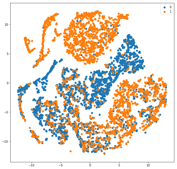
T-SNE visualization of hidden features for LSTM model trained on IMDB sentiment classification dataset

Please note that we reduced y_test_cat to 5000 instances too just like the tsne_results. You can change it and allow it to run longer.

Also, the classification report is shown for all the 25000 test instances. About 84% F1-score with a model trained for just 4 epochs. Cool! Here is the scatter plot we obtained.

As can be seen from the plot, the blue (0 — negative class) is fairly separable from the orange (1-positive class). Obviously, there are certain overlaps and the reason why our F-score is around 84 and not closer to 100 :). Understanding and visualizing the outputs at different layers can help understand which layer is causing major errors in learning representations.

I hope you find this article useful. I would love to hear your comments and thoughts. Also, do share your experiences with visualization.

Also, feel free to get in touch with me via LinkedIn.

 

 

 

 

 

来源： https://becominghuman.ai/visualizing-representations-bd9b62447e38

来自为知笔记(Wiz)