Caffe学习笔记4图像特征进行可视化

 

Caffe学习笔记4图像特征进行可视化

本文为原创作品，未经本人同意，禁止转载，禁止用于商业用途！本人对博客使用拥有最终解释权

 

欢迎关注我的博客：http://blog.csdn.net/hit2015spring和http://www.cnblogs.com/xujianqing/

 

这篇文章主要参考的是http://nbviewer.jupyter.org/github/BVLC/caffe/blob/master/examples/00-classification.ipynb

可以算是对它的翻译的总结吧，它可以算是学习笔记2的一个发展，2是介绍怎么提取特征，这是介绍怎么可视化特征

1、准备工作

首先安装依赖项

pip install cython

pip install h5py

pip install ipython

pip install leveldb

pip install matplotlib

pip install networkx

pip install nose

pip install numpy

pip install pandas

pip install protobuf

pip install python-gflags

pip install scikit-image

pip install scikit-learn

pip install scipy

接下来的操作都是在ipython中执行的，在ipython中用！表示执行shell命令，用$表示将python的变量转化为shell变量。通过这两种符号便可以实现shell命令和ipython的交互。

Ipython可以在终端运行，但是为了方便我们使用的是ipython notebook，这个玩意的介绍网上有很多的资源，这里就不赘述了，所以还要在你的主机上面配置ipython notebook

2、开始

2.1初始化并加载caffe

在终端输入

ipython notebook

新建一个文件

 

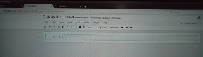
在终端输入代码，这里shift+enter表示运行代码，接下来每一个代码段输入完成后，运行一下！

# set up Python environment: numpy for numerical routines, and #matplotlib for plotting

import numpy as np

import matplotlib.pyplot as plt

# display plots in this notebook

%matplotlib inline

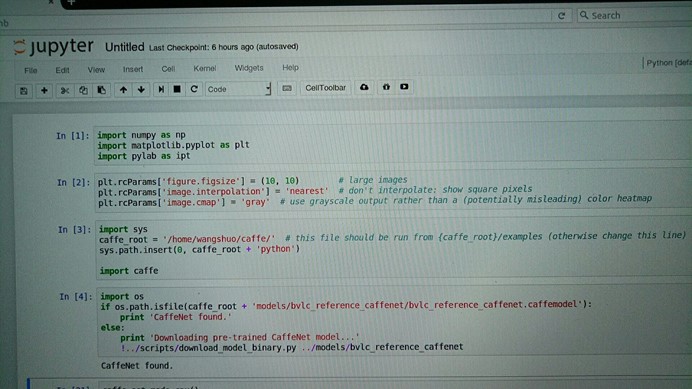
调入numpy子程序和matplotlib.pyplot（用于画图） 子程序，并将它们分别命名为np和plt

# set display defaults

plt.rcParams['figure.figsize'] = (10, 10) # large images

plt.rcParams['image.interpolation'] = 'nearest' # don't interpolate: show #square pixels

plt.rcParams['image.cmap'] = 'gray' # use grayscale output rather than #a (potentially misleading) color heatmap

设置显示图片的一些默认参数大小最大，图片插值原则为最近邻插值，图像为灰度图

# The caffe module needs to be on the Python path;

# we'll add it here explicitly.

import sys

caffe_root = '/home/wangshuo/caffe/' # this file should be run from {caffe_root}/examples (otherwise change this line)

sys.path.insert(0, caffe_root + 'python')

 

import caffe

# If you get "No module named _caffe", either you have not built pycaffe #or you have the wrong path.

加载caffe,把caffe的路径添加到当前的python路径下面来，如果没有添加路径，则会在python的路径下进行检索，会报错，caffe模块不存在。

import os

if os.path.isfile(caffe_root + 'models/bvlc_reference_caffenet/bvlc_reference_caffenet.caffemodel'):

print 'CaffeNet found.'

else:

print 'Downloading pre-trained CaffeNet model...'

!../scripts/download_model_binary.py ../models/bvlc_reference_caffenet

加载模型，这个模型在学习笔记1的时候已经下载过了，如果没有下载该模型可以用命令行

./examples/imagenet/get_caffe_reference_imagenet_model.sh

这里注意该模型的大小有233M左右，联网下载可能不全，注意查看，是个坑注意躲避！

2.2加载网络模型

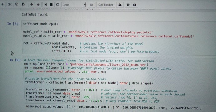
设置为cpu工作模式并加载网络模型

caffe.set_mode_cpu()

 

model_def = caffe_root + 'models/bvlc_reference_caffenet/deploy.prototxt'

model_weights = caffe_root + 'models/bvlc_reference_caffenet/bvlc_reference_caffenet.caffemodel'

 

net = caffe.Net(model_def, # defines the structure of the model

model_weights, # contains the trained weights

caffe.TEST) # use test mode (e.g., don't perform dropout)

model_def：定义模型的结构文件

model_weights：训练的权重

# load the mean ImageNet image (as distributed with Caffe) for subtraction

mu = np.load(caffe_root + 'python/caffe/imagenet/ilsvrc_2012_mean.npy')

mu = mu.mean(1).mean(1) # 获取BGR像素均值

print 'mean-subtracted values:', zip('BGR', mu)

 

# create transformer for the input called 'data'

transformer = caffe.io.Transformer({'data': net.blobs['data'].data.shape})

 

transformer.set_transpose('data', (2,0,1)) # move image channels to outermost dimension

transformer.set_mean('data', mu) # 各个通道的像素值减去图像均值

transformer.set_raw_scale('data', 255) # 设置灰度级为[0,255]而不是[0,1]

transformer.set_channel_swap('data', (2,1,0)) # 把RGB转为BGR

这段是设置输入的进行预处理，调用的是caffe.io.Transformer来进行预处理，这些预处理步骤是独立于其他的caffe部分的，所以可以使用传统的算法进行处理。

在caffe的默认设置中，使用的是BGR图像格式进行处理。像素的级数为[0,255],然后对这些图片进行预处理是减去均值，最后通道的信息会被转到第一个维度上来。

但是在matplotlib中加载的图片像素灰度级是[0,1]之间，且其通道数是在最里层的维度上的RGB格式故需要以上的转换

2.3CPU分类

# set the size of the input (we can skip this if we're happy

# with the default; we can also change it later, e.g., for different batch sizes)

net.blobs['data'].reshape(50, # 批次大小

3, # 3-channel (BGR) images

227, 227) # image size is 227x227

加载一个图片

image = caffe.io.load_image(caffe_root + 'examples/images/cat.jpg')

transformed_image = transformer.preprocess('data', image)

plt.imshow(image)

在这里运行完之后正常应该显示一张图片，然而并没有，具体看问题1

现在开始分类

# copy the image data into the memory allocated for the net

net.blobs['data'].data[...] = transformed_image

 

### perform classification

output = net.forward()

 

output_prob = output['prob'][0] # the output probability vector for the first image in the batch

 

print 'predicted class is:', output_prob.argmax()#分类输出最大概率的类别

输出：predicted class is: 281

第281类

但是我们需要更加准确地分类标签，因此加载分类标签

# load ImageNet labels

labels_file = caffe_root + 'data/ilsvrc12/synset_words.txt'

if not os.path.exists(labels_file):

!../data/ilsvrc12/get_ilsvrc_aux.sh

 

labels = np.loadtxt(labels_file, str, delimiter='\t')

 

print 'output label:', labels[output_prob.argmax()]

输出：output label: n02123045 tabby, tabby cat

判断准确，再看看把它判断成其他类别的输出概率：

# sort top five predictions from softmax output

top_inds = output_prob.argsort()[::-1][:5] # reverse sort and take five largest items

 

print 'probabilities and labels:'

zip(output_prob[top_inds], labels[top_inds])

输出：

probabilities and labels:

[(0.31243637, 'n02123045 tabby, tabby cat'),

(0.2379719, 'n02123159 tiger cat'),

(0.12387239, 'n02124075 Egyptian cat'),

(0.10075711, 'n02119022 red fox, Vulpes vulpes'),

(0.070957087, 'n02127052 lynx, catamount')]

可以看到最小的置信概率下输出的标签也比较明智

2.4切换到GPU模式

计算分类所用的时间，并把它和gpu模式比较

%timeit net.forward()

选择GPU模式

caffe.set_device(0) # if we have multiple GPUs, pick the first one

caffe.set_mode_gpu()

net.forward() # run once before timing to set up memory

%timeit net.forward()

3查看中间的输出

在每一层中我们主要关注的是激活的形状，它的典型格式为，批次，第二个是特征数，第三个第四个是每个神经元中图片的长宽

# for each layer, show the output shape

for layer_name, blob in net.blobs.iteritems():

print layer_name + '\t' + str(blob.data.shape)

查看每一层的输出形状

输出：

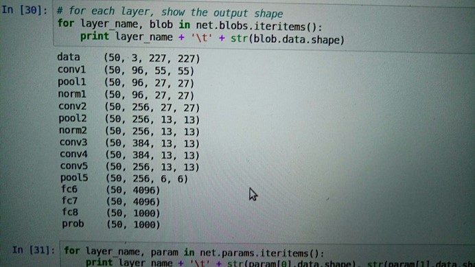
data    (50, 3, 227, 227)

conv1    (50, 96, 55, 55)

pool1    (50, 96, 27, 27)

norm1    (50, 96, 27, 27)

conv2    (50, 256, 27, 27)

pool2    (50, 256, 13, 13)

norm2    (50, 256, 13, 13)

conv3    (50, 384, 13, 13)

conv4    (50, 384, 13, 13)

conv5    (50, 256, 13, 13)

pool5    (50, 256, 6, 6)

fc6    (50, 4096)

fc7    (50, 4096)

fc8    (50, 1000)

prob    (50, 1000)

再看看参数的结构，参数结构是被另外一个函数定义的选择输出的类型，0代表权重，1代表偏差，权重有4维特征（输出的通道数，输入通道数，滤波的高，滤波的宽），偏差有一维（输出的通道）

for layer_name, param in net.params.iteritems():

print layer_name + '\t' + str(param[0].data.shape), str(param[1].data.shape)

对这些特征进行可视化：定义一个函数

def vis_square(data):

"""Take an array of shape (n, height, width) or (n, height, width, 3)

and visualize each (height, width) thing in a grid of size approx. sqrt(n) by sqrt(n)"""

 

# normalize data for display

data = (data - data.min()) / (data.max() - data.min())

 

# force the number of filters to be square

n = int(np.ceil(np.sqrt(data.shape[0])))

padding = (((0, n ** 2 - data.shape[0]),

(0, 1), (0, 1)) # add some space between filters

+ ((0, 0),) * (data.ndim - 3)) # don't pad the last dimension (if there is one)

data = np.pad(data, padding, mode='constant', constant_values=1) # pad with ones (white)

 

# tile the filters into an image

data = data.reshape((n, n) + data.shape[1:]).transpose((0, 2, 1, 3) + tuple(range(4, data.ndim + 1)))

data = data.reshape((n * data.shape[1], n * data.shape[3]) + data.shape[4:])

ipt.show()

plt.imshow(data); plt.axis('off')

显示第一个卷积层的特征

# the parameters are a list of [weights, biases]

filters = net.params['conv1'][0].data

vis_square(filters.transpose(0, 2, 3, 1))

 

遇到问题

在运行plt.imshow(image)之后应该显示相应的图片，最后没有显示，这里有一个问题就是，需要在导入nump的时候也要导入pylab

import pylab as ipt

在显示之前添上

ipt.show()

所以问题1的答案为

image = caffe.io.load_image(caffe_root + 'examples/images/cat.jpg')

transformed_image = transformer.preprocess('data', image)

ipt.show()

plt.imshow(image)