Deep learning：四十八(Contractive AutoEncoder简单理解)

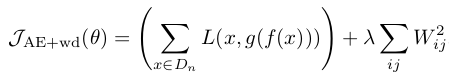
　　Contractive autoencoder是autoencoder的一个变种，其实就是在autoencoder上加入了一个规则项，它简称CAE（对应中文翻译为？）。通常情况下，对权值进行惩罚后的autoencoder数学表达形式为：

　　

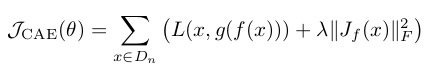
　　这是直接对W的值进行惩罚的，而今天要讲的CAE其数学表达式同样非常简单，如下：

　　

　　其中的 是隐含层输出值关于权重的雅克比矩阵，而  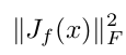 表示的是该雅克比矩阵的F范数的平方，即雅克比矩阵中每个元素求平方

　　

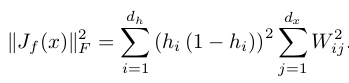
　　然后求和，更具体的数学表达式为：

　　

　　关于雅克比矩阵的介绍可参考雅克比矩阵&行列式——单纯的矩阵和算子，关于F范数可参考我前面的博文Sparse coding中关于矩阵的范数求导中的内容。

　　有了loss函数的表达式，采用常见的mini-batch随机梯度下降法训练即可。

　　关于为什么contrative autoencoder效果这么好？paper中作者解释了好几页，好吧，我真没完全明白，希望懂的朋友能简单通俗的介绍下。下面是读完文章中的一些理解：

　　好的特征表示大致有2个衡量标准：1. 可以很好的重构出输入数据; 2.对输入数据一定程度下的扰动具有不变形。普通的autoencoder和sparse autoencoder主要是符合第一个标准。而deniose autoencoder和contractive autoencoder则主要体现在第二个。而作为分类任务来说，第二个标准显得更重要。

　　雅克比矩阵包含数据在各种方向上的信息，可以对雅克比矩阵进行奇异值分解，同时画出奇异值数目和奇异值的曲线图，大的奇异值对应着学习到的局部方向可允许的变化量，并且曲线越抖越好（这个图没看明白，所以这里的解释基本上是直接翻译原文中某些观点）。

　　另一个曲线图是contractive ratio图，contractive ratio定义为：原空间中2个样本直接的距离比上特征空间（指映射后的空间）中对应2个样本点之间的距离。某个点x处局部映射的contraction值是指该点处雅克比矩阵的F范数。按照作者的观点，contractive ration曲线呈上升趋势的话更好（why？），而CAE刚好符合。

　　总之Contractive autoencoder主要是抑制训练样本（处在低维流形曲面上）在所有方向上的扰动。

　　CAE的代码可参考：pylearn2/cA.py 　　

"""This tutorial introduces Contractive auto-encoders (cA) using Theano.

 They are based on auto-encoders as the ones used in Bengio et
 al. 2007.  An autoencoder takes an input x and first maps it to a
 hidden representation y = f_{\theta}(x) = s(Wx+b), parameterized by
 \theta={W,b}. The resulting latent representation y is then mapped
 back to a "reconstructed" vector z \in [0,1]^d in input space z =
 g_{\theta'}(y) = s(W'y + b').  The weight matrix W' can optionally be
 constrained such that W' = W^T, in which case the autoencoder is said
 to have tied weights. The network is trained such that to minimize
 the reconstruction error (the error between x and z).  Adding the
 squared Frobenius norm of the Jacobian of the hidden mapping h with
 respect to the visible units yields the contractive auto-encoder:

      - \sum_{k=1}^d[ x_k \log z_k + (1-x_k) \log( 1-z_k)]  + \| \frac{\partial h(x)}{\partial x} \|^2

 References :
   - S. Rifai, P. Vincent, X. Muller, X. Glorot, Y. Bengio: Contractive
   Auto-Encoders: Explicit Invariance During Feature Extraction, ICML-11

   - S. Rifai, X. Muller, X. Glorot, G. Mesnil, Y. Bengio, and Pascal
     Vincent. Learning invariant features through local space
     contraction. Technical Report 1360, Universite de Montreal

   - Y. Bengio, P. Lamblin, D. Popovici, H. Larochelle: Greedy Layer-Wise
   Training of Deep Networks, Advances in Neural Information Processing
   Systems 19, 2007

"""
import cPickle
import gzip
import os
import sys
import time

import numpy

import theano
import theano.tensor as T

from logistic_sgd import load_data
from utils import tile_raster_images

import PIL.Image

class cA(object):
    """ Contractive Auto-Encoder class (cA)

    The contractive autoencoder tries to reconstruct the input with an
    additional constraint on the latent space. With the objective of
    obtaining a robust representation of the input space, we
    regularize the L2 norm(Froebenius) of the jacobian of the hidden
    representation with respect to the input. Please refer to Rifai et
    al.,2011 for more details.

    If x is the input then equation (1) computes the projection of the
    input into the latent space h. Equation (2) computes the jacobian
    of h with respect to x.  Equation (3) computes the reconstruction
    of the input, while equation (4) computes the reconstruction
    error and the added regularization term from Eq.(2).

    .. math::

        h_i = s(W_i x + b_i)                                             (1)

        J_i = h_i (1 - h_i) * W_i                                        (2)

        x' = s(W' h  + b')                                               (3)

        L = -sum_{k=1}^d [x_k \log x'_k + (1-x_k) \log( 1-x'_k)]
             + lambda * sum_{i=1}^d sum_{j=1}^n J_{ij}^2                 (4)

    """

    def __init__(self, numpy_rng, input=None, n_visible=784, n_hidden=100,
                 n_batchsize=1, W=None, bhid=None, bvis=None):
        """Initialize the cA class by specifying the number of visible units (the
        dimension d of the input ), the number of hidden units ( the dimension
        d' of the latent or hidden space ) and the contraction level. The
        constructor also receives symbolic variables for the input, weights and
        bias.

        :type numpy_rng: numpy.random.RandomState
        :param numpy_rng: number random generator used to generate weights

        :type theano_rng: theano.tensor.shared_randomstreams.RandomStreams
        :param theano_rng: Theano random generator; if None is given
                     one is generated based on a seed drawn from `rng`

        :type input: theano.tensor.TensorType
        :param input: a symbolic description of the input or None for
                      standalone cA

        :type n_visible: int
        :param n_visible: number of visible units

        :type n_hidden: int
        :param n_hidden:  number of hidden units

        :type n_batchsize int
        :param n_batchsize: number of examples per batch

        :type W: theano.tensor.TensorType
        :param W: Theano variable pointing to a set of weights that should be
                  shared belong the dA and another architecture; if dA should
                  be standalone set this to None

        :type bhid: theano.tensor.TensorType
        :param bhid: Theano variable pointing to a set of biases values (for
                     hidden units) that should be shared belong dA and another
                     architecture; if dA should be standalone set this to None

        :type bvis: theano.tensor.TensorType
        :param bvis: Theano variable pointing to a set of biases values (for
                     visible units) that should be shared belong dA and another
                     architecture; if dA should be standalone set this to None

        """
        self.n_visible = n_visible
        self.n_hidden = n_hidden
        self.n_batchsize = n_batchsize
        # note : W' was written as `W_prime` and b' as `b_prime`
        if not W:
            # W is initialized with `initial_W` which is uniformely sampled
            # from -4*sqrt(6./(n_visible+n_hidden)) and
            # 4*sqrt(6./(n_hidden+n_visible))the output of uniform if
            # converted using asarray to dtype
            # theano.config.floatX so that the code is runable on GPU
            initial_W = numpy.asarray(numpy_rng.uniform(
                      low=-4 * numpy.sqrt(6. / (n_hidden + n_visible)),
                      high=4 * numpy.sqrt(6. / (n_hidden + n_visible)),
                      size=(n_visible, n_hidden)),
                                      dtype=theano.config.floatX)
            W = theano.shared(value=initial_W, name='W', borrow=True)

        if not bvis:
            bvis = theano.shared(value=numpy.zeros(n_visible,
                                                   dtype=theano.config.floatX),
                                 borrow=True)

        if not bhid:
            bhid = theano.shared(value=numpy.zeros(n_hidden,
                                                   dtype=theano.config.floatX),
                                 name='b',
                                 borrow=True)

        self.W = W
        # b corresponds to the bias of the hidden
        self.b = bhid
        # b_prime corresponds to the bias of the visible
        self.b_prime = bvis
        # tied weights, therefore W_prime is W transpose
        self.W_prime = self.W.T

        # if no input is given, generate a variable representing the input
        if input == None:
            # we use a matrix because we expect a minibatch of several
            # examples, each example being a row
            self.x = T.dmatrix(name='input')
        else:
            self.x = input

        self.params = [self.W, self.b, self.b_prime]

    def get_hidden_values(self, input): #激发函数为sigmoid看，这里只向前进一次
        """ Computes the values of the hidden layer """
        return T.nnet.sigmoid(T.dot(input, self.W) + self.b)

    def get_jacobian(self, hidden, W):
        """Computes the jacobian of the hidden layer with respect to
        the input, reshapes are necessary for broadcasting the
        element-wise product on the right axis

        """
        return T.reshape(hidden * (1 - hidden), #计算雅克比矩阵，先将h(1-h)变成3维矩阵，然后将w也变成3维矩阵，然后将这2个3维矩阵
                         (self.n_batchsize, 1, self.n_hidden)) * T.reshape( #对应元素相乘，但怎么感觉2个矩阵尺寸不对应呢？
                             W, (1, self.n_visible, self.n_hidden))

    def get_reconstructed_input(self, hidden): #重构输入时获得的输出端数据
        """Computes the reconstructed input given the values of the
        hidden layer

        """
        return  T.nnet.sigmoid(T.dot(hidden, self.W_prime) + self.b_prime)

    def get_cost_updates(self, contraction_level, learning_rate):
        """ This function computes the cost and the updates for one trainng
        step of the cA """

        y = self.get_hidden_values(self.x)
        z = self.get_reconstructed_input(y)
        J = self.get_jacobian(y, self.W)
        # note : we sum over the size of a datapoint; if we are using
        #        minibatches, L will be a vector, with one entry per
        #        example in minibatch
        self.L_rec = - T.sum(self.x * T.log(z) + #交叉熵作为重构误差(当输入是[0,1],且是sigmoid时可以采用)
                             (1 - self.x) * T.log(1 - z),
                             axis=1)

        # Compute the jacobian and average over the number of samples/minibatch
        self.L_jacob = T.sum(J ** 2) / self.n_batchsize

        # note : L is now a vector, where each element is the
        #        cross-entropy cost of the reconstruction of the
        #        corresponding example of the minibatch. We need to
        #        compute the average of all these to get the cost of
        #        the minibatch
        cost = T.mean(self.L_rec) + contraction_level * T.mean(self.L_jacob)

        # compute the gradients of the cost of the `cA` with respect
        # to its parameters
        gparams = T.grad(cost, self.params) #Theano特有的功能，自动求导
        # generate the list of updates
        updates = []
        for param, gparam in zip(self.params, gparams):
            updates.append((param, param - learning_rate * gparam)) #SGD算法 

        return (cost, updates)

def test_cA(learning_rate=0.01, training_epochs=20,
            dataset='./data/mnist.pkl.gz',
            batch_size=10, output_folder='cA_plots', contraction_level=.1):
    """
    This demo is tested on MNIST

    :type learning_rate: float
    :param learning_rate: learning rate used for training the contracting
                          AutoEncoder

    :type training_epochs: int
    :param training_epochs: number of epochs used for training

    :type dataset: string
    :param dataset: path to the picked dataset

    """
    datasets = load_data(dataset)
    train_set_x, train_set_y = datasets[0]

    # compute number of minibatches for training, validation and testing
    n_train_batches = train_set_x.get_value(borrow=True).shape[0] / batch_size #标识borrow=True表示不需要复制样本

    # allocate symbolic variables for the data
    index = T.lscalar()    # index to a [mini]batch
    x = T.matrix('x')  # the data is presented as rasterized images

    if not os.path.isdir(output_folder):
        os.makedirs(output_folder)
    os.chdir(output_folder)
    ####################################
    #        BUILDING THE MODEL        #
    ####################################

    rng = numpy.random.RandomState(123)

    ca = cA(numpy_rng=rng, input=x,
            n_visible=28 * 28, n_hidden=500, n_batchsize=batch_size) #500个隐含层节点

    cost, updates = ca.get_cost_updates(contraction_level=contraction_level, #update里面装的是参数的更新过程
                                        learning_rate=learning_rate)

    train_ca = theano.function([index], [T.mean(ca.L_rec), ca.L_jacob], #定义函数，输入为batch的索引，输出为该batch下的重构误差和雅克比误差
                               updates=updates,
                               givens={x: train_set_x[index * batch_size:
                                                    (index + 1) * batch_size]})

    start_time = time.clock()

    ############
    # TRAINING #
    ############

    # go through training epochs
    for epoch in xrange(training_epochs): #循环20次
        # go through trainng set
        c = []
        for batch_index in xrange(n_train_batches):
            c.append(train_ca(batch_index)) #计算loss值,计算过程中其实也一直在更新updates权值

        c_array = numpy.vstack(c) #vstack()为将矩阵序列c按照每行叠加，重新构造一个矩阵
        print 'Training epoch %d, reconstruction cost ' % epoch, numpy.mean(
            c_array[0]), ' jacobian norm ', numpy.mean(numpy.sqrt(c_array[1]))

    end_time = time.clock()

    training_time = (end_time - start_time)
    #下面是显示和保存学习到的权值结果
    print >> sys.stderr, ('The code for file ' + os.path.split(__file__)[1] +
                          ' ran for %.2fm' % ((training_time) / 60.))
    image = PIL.Image.fromarray(tile_raster_images(
        X=ca.W.get_value(borrow=True).T,
        img_shape=(28, 28), tile_shape=(10, 10),
        tile_spacing=(1, 1)))

    image.save('cae_filters.png')

    os.chdir('../')

if __name__ == '__main__':
    test_cA()

　　按照原程序，迭代20次，跑了6个多小时，重构误差项和contraction项变化情况如下：

... loading data
Training epoch 0, reconstruction cost  589.571872577  jacobian norm  20.9938791886
Training epoch 1, reconstruction cost  115.13390224  jacobian norm  10.673699659
Training epoch 2, reconstruction cost  101.291018001  jacobian norm  10.134422748
Training epoch 3, reconstruction cost  94.220284334  jacobian norm  9.84685383242
Training epoch 4, reconstruction cost  89.5890225412  jacobian norm  9.64736166807
Training epoch 5, reconstruction cost  86.1490384385  jacobian norm  9.49857669084
Training epoch 6, reconstruction cost  83.4664242016  jacobian norm  9.38143172793
Training epoch 7, reconstruction cost  81.3512907826  jacobian norm  9.28327421556
Training epoch 8, reconstruction cost  79.6482831506  jacobian norm  9.19748922967
Training epoch 9, reconstruction cost  78.2066659332  jacobian norm  9.12143982155
Training epoch 10, reconstruction cost  76.9456192804  jacobian norm  9.05343287129
Training epoch 11, reconstruction cost  75.8435863545  jacobian norm  8.99151663486
Training epoch 12, reconstruction cost  74.8999458491  jacobian norm  8.9338049163
Training epoch 13, reconstruction cost  74.1060022563  jacobian norm  8.87925367541
Training epoch 14, reconstruction cost  73.4415396294  jacobian norm  8.8291852146
Training epoch 15, reconstruction cost  72.879630175  jacobian norm  8.78442892358
Training epoch 16, reconstruction cost  72.3729563995  jacobian norm  8.74324402838
Training epoch 17, reconstruction cost  71.8622392555  jacobian norm  8.70262903409
Training epoch 18, reconstruction cost  71.3049790204  jacobian norm  8.66103980493
Training epoch 19, reconstruction cost  70.6462751293  jacobian norm  8.61777944201

　　参考资料：

Contractive auto-encoders: Explicit invariance during feature extraction，Salah Rifai，Pascal Vincent，Xavier Muller，Xavier Glorot，Yoshua Bengio

　  雅克比矩阵&行列式——单纯的矩阵和算子

　  Sparse coding中关于矩阵的范数求导

pylearn2/cA.py

再谈雅克比矩阵---在feature learning中的作用