利用python深度学习算法来绘图

可以画画啊！可以画画啊！可以画画啊！ 对，有趣的事情需要讲三遍。
事情是这样的，通过python的深度学习算法包去训练计算机模仿世界名画的风格，然后应用到另一幅画中，不多说直接上图！

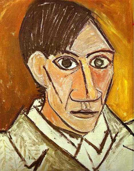
&lt;img src="https://pic3.zhimg.com/50/98cab4f35d2084f969a8189e90b47dee_hd.jpg" data-rawwidth="468" data-rawheight="600" class="origin_image zh-lightbox-thumb" width="468" data-original="https://pic3.zhimg.com/98cab4f35d2084f969a8189e90b47dee_r.jpg"&gt;

这个是世界名画”毕加索的自画像“（我也不懂什么是世界名画，但是我会google呀哈哈），以这张图片为模板，让计算机去学习这张图片的风格（至于怎么学习请参照这篇国外大牛的论文http://arxiv.org/abs/1508.06576）应用到自己的这张图片上。

&lt;img src="https://pic2.zhimg.com/50/7ca4eb6c6088ad9880a4bc1a9993ed35_hd.jpg" data-rawwidth="249" data-rawheight="365" class="content_image" width="249"&gt;

结果就变成下面这个样子了

&lt;img src="https://pic1.zhimg.com/50/b869feb93320634a2c05752efd02bc74_hd.png" data-rawwidth="472" data-rawheight="660" class="origin_image zh-lightbox-thumb" width="472" data-original="https://pic1.zhimg.com/b869feb93320634a2c05752efd02bc74_r.png"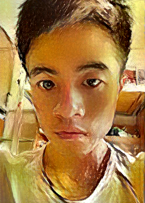&gt;

咦，吓死宝宝了，不过好玩的东西当然要身先士卒啦！
接着由于距离开学也越来越近了，为了给广大新生营造一个良好的校园，噗！为了美化校园在新生心目中的形象学长真的不是有意要欺骗你们的。特意制作了下面的《梵高笔下的东华理工大学》，是不是没有听说过这个大学，的确她就是一个普通的二本学校不过这都不是重点。
左边的图片是梵高的《星空》作为模板，中间的图片是待转化的图片，右边的图片是结果

&lt;img src="https://pic2.zhimg.com/50/16b2c1522cea0ae43c4d2c1cc6871b29_hd.png" data-rawwidth="852" data-rawheight="172" class="origin_image zh-lightbox-thumb" width="852" data-original="https://pic2.zhimg.com/16b2c1522cea0ae43c4d2c1cc6871b29_r.png"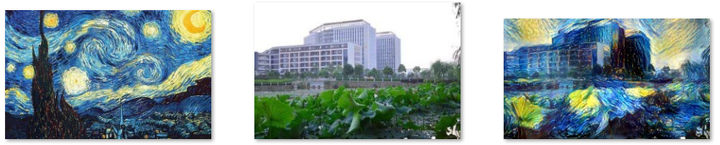&gt;

这是我们学校的内“湖”（池塘）

&lt;img src="https://pic1.zhimg.com/50/193695070e8614fb75b4735ad2d68734_hd.png" data-rawwidth="856" data-rawheight="173" class="origin_image zh-lightbox-thumb" width="856" data-original="https://pic1.zhimg.com/193695070e8614fb75b4735ad2d68734_r.png"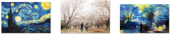&gt;

校园里的樱花广场（个人觉得这是我校最浪漫的地方了）

&lt;img src="https://pic3.zhimg.com/50/dd333413cb332f5d0681ba479249f802_hd.png" data-rawwidth="848" data-rawheight="206" class="origin_image zh-lightbox-thumb" width="848" data-original="https://pic3.zhimg.com/dd333413cb332f5d0681ba479249f802_r.png"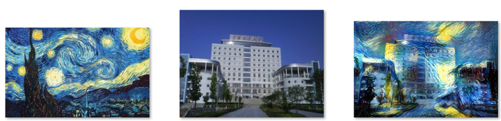&gt;

不多说，学校图书馆

&lt;img src="https://pic4.zhimg.com/50/9029082a8fdb697873f7250d0137a617_hd.png" data-rawwidth="851" data-rawheight="194" class="origin_image zh-lightbox-thumb" width="851" data-original="https://pic4.zhimg.com/9029082a8fdb697873f7250d0137a617_r.png"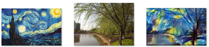&gt;

“池塘”边的柳树

&lt;img src="https://pic1.zhimg.com/50/8d8dcbca85b62f276129d6d237d4d6fc_hd.png" data-rawwidth="852" data-rawheight="204" class="origin_image zh-lightbox-thumb" width="852" data-original="https://pic1.zhimg.com/8d8dcbca85b62f276129d6d237d4d6fc_r.png"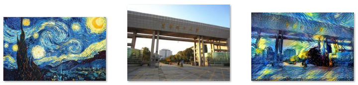&gt;

学校东大门

&lt;img src="https://pic1.zhimg.com/50/ad22383f37f56d92517b18bb830ee7c8_hd.png" data-rawwidth="862" data-rawheight="164" class="origin_image zh-lightbox-thumb" width="862" data-original="https://pic1.zhimg.com/ad22383f37f56d92517b18bb830ee7c8_r.png"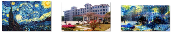&gt;

学校测绘楼

&lt;img src="https://pic3.zhimg.com/50/cb6d76286324c857528892014d04bb3e_hd.png" data-rawwidth="852" data-rawheight="211" class="origin_image zh-lightbox-thumb" width="852" data-original="https://pic3.zhimg.com/cb6d76286324c857528892014d04bb3e_r.png"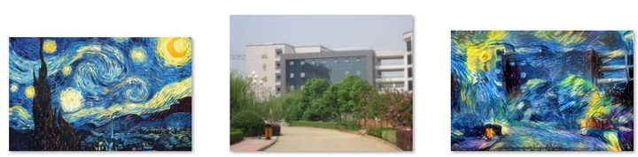&gt;

学校地学楼

为了便于观看，附上生成后的大图：

&lt;img src="https://pic3.zhimg.com/50/d7ee30ae90b3d81049abee478e8e75b6_hd.png" data-rawwidth="699" data-rawheight="408" class="origin_image zh-lightbox-thumb" width="699" data-original="https://pic3.zhimg.com/d7ee30ae90b3d81049abee478e8e75b6_r.png"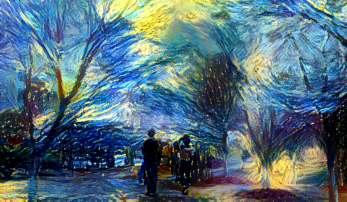&gt;
&lt;img src="https://pic3.zhimg.com/50/c04d56309b493bd2a0d3db26d0916206_hd.png" data-rawwidth="700" data-rawheight="465" class="origin_image zh-lightbox-thumb" width="700" data-original="https://pic3.zhimg.com/c04d56309b493bd2a0d3db26d0916206_r.png"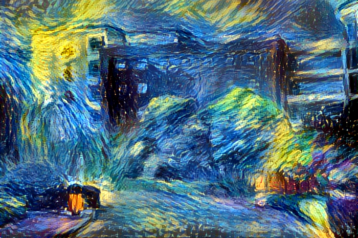&gt;
&lt;img src="https://pic1.zhimg.com/50/f41d8d145b8a8fe30abba37ede85c778_hd.png" data-rawwidth="695" data-rawheight="370" class="origin_image zh-lightbox-thumb" width="695" data-original="https://pic1.zhimg.com/f41d8d145b8a8fe30abba37ede85c778_r.png"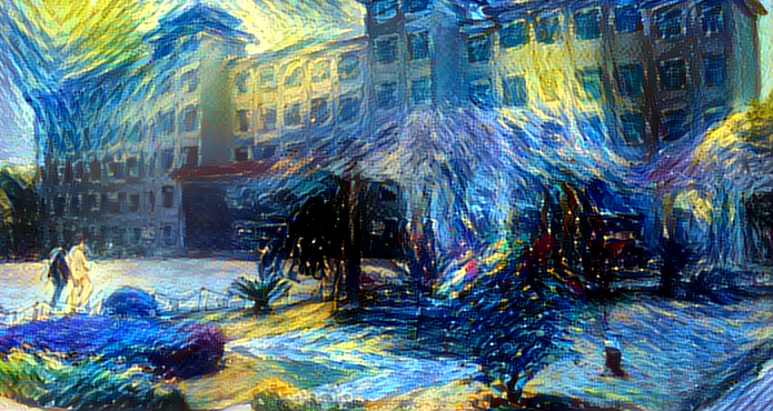&gt;
&lt;img src="https://pic1.zhimg.com/50/797a561056109585428a10c9a6278874_hd.png" data-rawwidth="700" data-rawheight="447" class="origin_image zh-lightbox-thumb" width="700" data-original="https://pic1.zhimg.com/797a561056109585428a10c9a6278874_r.png"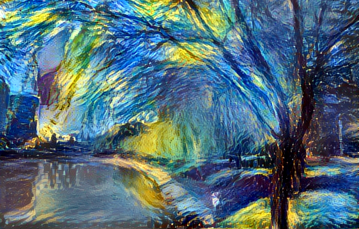&gt;
&lt;img src="https://pic1.zhimg.com/50/d4e2ac5460d08d0cd9af15bc154574e4_hd.png" data-rawwidth="699" data-rawheight="469" class="origin_image zh-lightbox-thumb" width="699" data-original="https://pic1.zhimg.com/d4e2ac5460d08d0cd9af15bc154574e4_r.png"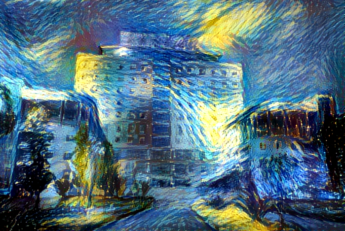&gt;
&lt;img src="https://pic4.zhimg.com/50/7ea97eab41a2c2eb32d356b1afd9ca2f_hd.png" data-rawwidth="698" data-rawheight="409" class="origin_image zh-lightbox-thumb" width="698" data-original="https://pic4.zhimg.com/7ea97eab41a2c2eb32d356b1afd9ca2f_r.png"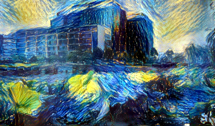&gt;
&lt;img src="https://pic1.zhimg.com/50/5f1f741537b28b9ec9e0d6e66b76a2cc_hd.png" data-rawwidth="699" data-rawheight="469" class="origin_image zh-lightbox-thumb" width="699" data-original="https://pic1.zhimg.com/5f1f741537b28b9ec9e0d6e66b76a2cc_r.png"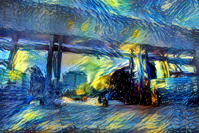&gt;

别看才区区七张图片，可是这让计算机运行了好长的时间，期间电脑死机两次！

好了广告打完了，下面是福利时间

在本地用keras搭建风格转移平台

1.相关依赖库的安装

# 命令行安装keras、h5py、tensorflow

pip3 install keras

pip3 install h5py

pip3 install tensorflow

如果tensorflowan命令行安装失败，可以在这里下载whl包Python Extension Packages for Windows （进入网址后ctrl+F输入tensorflow可以快速搜索）

2.配置运行环境

下载VGG16模型 https://pan.baidu.com/s/1i5wYN1z 放入如下目录当中

&lt;img src="https://pic1.zhimg.com/50/v2-b06fa971e3b6ebc905097f89be3ce39c_hd.png" data-rawwidth="654" data-rawheight="129" class="origin_image zh-lightbox-thumb" width="654" data-original="https://pic1.zhimg.com/v2-b06fa971e3b6ebc905097f89be3ce39c_r.png"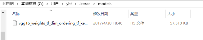&gt;

3.代码编写

from __future__ import print_function

from keras.preprocessing.image import load_img, img_to_array

from scipy.misc import imsave

import numpy as np

from scipy.optimize import fmin_l_bfgs_b

import time

import argparse

from keras.applications import vgg16

from keras import backend as K

parser = argparse.ArgumentParser(description='Neural style transfer with Keras.')

parser.add_argument('base_image_path', metavar='base', type=str,

                    help='Path to the image to transform.')

parser.add_argument('style_reference_image_path', metavar='ref', type=str,

                    help='Path to the style reference image.')

parser.add_argument('result_prefix', metavar='res_prefix', type=str,

                    help='Prefix for the saved results.')

parser.add_argument('--iter', type=int, default=10, required=False,

                    help='Number of iterations to run.')

parser.add_argument('--content_weight', type=float, default=0.025, required=False,

                    help='Content weight.')

parser.add_argument('--style_weight', type=float, default=1.0, required=False,

                    help='Style weight.')

parser.add_argument('--tv_weight', type=float, default=1.0, required=False,

                    help='Total Variation weight.')

args = parser.parse_args()

base_image_path = args.base_image_path

style_reference_image_path = args.style_reference_image_path

result_prefix = args.result_prefix

iterations = args.iter

# these are the weights of the different loss components

total_variation_weight = args.tv_weight

style_weight = args.style_weight

content_weight = args.content_weight

# dimensions of the generated picture.

width, height = load_img(base_image_path).size

img_nrows = 400

img_ncols = int(width * img_nrows / height)

# util function to open, resize and format pictures into appropriate tensors

def preprocess_image(image_path):

    img = load_img(image_path, target_size=(img_nrows, img_ncols))

    img = img_to_array(img)

    img = np.expand_dims(img, axis=0)

    img = vgg16.preprocess_input(img)

    return img

# util function to convert a tensor into a valid image

def deprocess_image(x):

    if K.image_data_format() == 'channels_first':

        x = x.reshape((3, img_nrows, img_ncols))

        x = x.transpose((1, 2, 0))

    else:

        x = x.reshape((img_nrows, img_ncols, 3))

    # Remove zero-center by mean pixel

    x[:, :, 0] += 103.939

    x[:, :, 1] += 116.779

    x[:, :, 2] += 123.68

    # 'BGR'->'RGB'

    x = x[:, :, ::-1]

    x = np.clip(x, 0, 255).astype('uint8')

    return x

# get tensor representations of our images

base_image = K.variable(preprocess_image(base_image_path))

style_reference_image = K.variable(preprocess_image(style_reference_image_path))

# this will contain our generated image

if K.image_data_format() == 'channels_first':

    combination_image = K.placeholder((1, 3, img_nrows, img_ncols))

else:

    combination_image = K.placeholder((1, img_nrows, img_ncols, 3))

# combine the 3 images into a single Keras tensor

input_tensor = K.concatenate([base_image,

                              style_reference_image,

                              combination_image], axis=0)

# build the VGG16 network with our 3 images as input

# the model will be loaded with pre-trained ImageNet weights

model = vgg16.VGG16(input_tensor=input_tensor,

                    weights='imagenet', include_top=False)

print('Model loaded.')

# get the symbolic outputs of each "key" layer (we gave them unique names).

outputs_dict = dict([(layer.name, layer.output) for layer in model.layers])

# compute the neural style loss

# first we need to define 4 util functions

# the gram matrix of an image tensor (feature-wise outer product)

def gram_matrix(x):

    assert K.ndim(x) == 3

    if K.image_data_format() == 'channels_first':

        features = K.batch_flatten(x)

    else:

        features = K.batch_flatten(K.permute_dimensions(x, (2, 0, 1)))

    gram = K.dot(features, K.transpose(features))

    return gram

# the "style loss" is designed to maintain

# the style of the reference image in the generated image.

# It is based on the gram matrices (which capture style) of

# feature maps from the style reference image

# and from the generated image

def style_loss(style, combination):

    assert K.ndim(style) == 3

    assert K.ndim(combination) == 3

    S = gram_matrix(style)

    C = gram_matrix(combination)

    channels = 3

    size = img_nrows * img_ncols

    return K.sum(K.square(S - C)) / (4. * (channels ** 2) * (size ** 2))

# an auxiliary loss function

# designed to maintain the "content" of the

# base image in the generated image

def content_loss(base, combination):

    return K.sum(K.square(combination - base))

# the 3rd loss function, total variation loss,

# designed to keep the generated image locally coherent

def total_variation_loss(x):

    assert K.ndim(x) == 4

    if K.image_data_format() == 'channels_first':

        a = K.square(x[:, :, :img_nrows - 1, :img_ncols - 1] - x[:, :, 1:, :img_ncols - 1])

        b = K.square(x[:, :, :img_nrows - 1, :img_ncols - 1] - x[:, :, :img_nrows - 1, 1:])

    else:

        a = K.square(x[:, :img_nrows - 1, :img_ncols - 1, :] - x[:, 1:, :img_ncols - 1, :])

        b = K.square(x[:, :img_nrows - 1, :img_ncols - 1, :] - x[:, :img_nrows - 1, 1:, :])

    return K.sum(K.pow(a + b, 1.25))

# combine these loss functions into a single scalar

loss = K.variable(0.)

layer_features = outputs_dict['block4_conv2']

base_image_features = layer_features[0, :, :, :]

combination_features = layer_features[2, :, :, :]

loss += content_weight * content_loss(base_image_features,

                                      combination_features)

feature_layers = ['block1_conv1', 'block2_conv1',

                  'block3_conv1', 'block4_conv1',

                  'block5_conv1']

for layer_name in feature_layers:

    layer_features = outputs_dict[layer_name]

    style_reference_features = layer_features[1, :, :, :]

    combination_features = layer_features[2, :, :, :]

    sl = style_loss(style_reference_features, combination_features)

    loss += (style_weight / len(feature_layers)) * sl

loss += total_variation_weight * total_variation_loss(combination_image)

# get the gradients of the generated image wrt the loss

grads = K.gradients(loss, combination_image)

outputs = [loss]

if isinstance(grads, (list, tuple)):

    outputs += grads

else:

    outputs.append(grads)

f_outputs = K.function([combination_image], outputs)

def eval_loss_and_grads(x):

    if K.image_data_format() == 'channels_first':

        x = x.reshape((1, 3, img_nrows, img_ncols))

    else:

        x = x.reshape((1, img_nrows, img_ncols, 3))

    outs = f_outputs([x])

    loss_value = outs[0]

    if len(outs[1:]) == 1:

        grad_values = outs[1].flatten().astype('float64')

    else:

        grad_values = np.array(outs[1:]).flatten().astype('float64')

    return loss_value, grad_values

# this Evaluator class makes it possible

# to compute loss and gradients in one pass

# while retrieving them via two separate functions,

# "loss" and "grads". This is done because scipy.optimize

# requires separate functions for loss and gradients,

# but computing them separately would be inefficient.

class Evaluator(object):

    def __init__(self):

        self.loss_value = None

        self.grads_values = None

    def loss(self, x):

        assert self.loss_value is None

        loss_value, grad_values = eval_loss_and_grads(x)

        self.loss_value = loss_value

        self.grad_values = grad_values

        return self.loss_value

    def grads(self, x):

        assert self.loss_value is not None

        grad_values = np.copy(self.grad_values)

        self.loss_value = None

        self.grad_values = None

        return grad_values

evaluator = Evaluator()

# run scipy-based optimization (L-BFGS) over the pixels of the generated image

# so as to minimize the neural style loss

if K.image_data_format() == 'channels_first':

    x = np.random.uniform(0, 255, (1, 3, img_nrows, img_ncols)) - 128.

else:

    x = np.random.uniform(0, 255, (1, img_nrows, img_ncols, 3)) - 128.

for i in range(iterations):

    print('Start of iteration', i)

    start_time = time.time()

    x, min_val, info = fmin_l_bfgs_b(evaluator.loss, x.flatten(),

                                     fprime=evaluator.grads, maxfun=20)

    print('Current loss value:', min_val)

    # save current generated image

    img = deprocess_image(x.copy())

    fname = result_prefix + '_at_iteration_%d.png' % i

    imsave(fname, img)

    end_time = time.time()

    print('Image saved as', fname)

print('Iteration %d completed in %ds' % (i, end_time - start_time))

复制上述代码保存为neural_style_transfer.py(随便命名)

4.运行

新建一个空文件夹，把上一步骤的文件neural_style_transfer.py放入这个空文件夹中。然后把相应的模板图片，待转化图片放入该文件当中。

python neural_style_transfer.py   你的待转化图片路径    模板图片路径   保存的生产图片路径加名称（注意不需要有.jpg等后缀）

 python neural_style_transfer.py './me.jpg' './starry_night.jpg' './me_t'

迭代结果截图：

&lt;img src="https://pic3.zhimg.com/50/v2-7bd28bae3b546a72d56e0e3d568152b2_hd.png" data-rawwidth="484" data-rawheight="595" class="origin_image zh-lightbox-thumb" width="484" data-original="https://pic3.zhimg.com/v2-7bd28bae3b546a72d56e0e3d568152b2_r.png"&gt;

迭代过程对比

&lt;img src="https://pic3.zhimg.com/50/v2-325064dfc72b82872a4a70a4f87ef1e6_hd.png" data-rawwidth="778" data-rawheight="496" class="origin_image zh-lightbox-thumb" width="778" data-original="https://pic3.zhimg.com/v2-325064dfc72b82872a4a70a4f87ef1e6_r.png"&gt;

其它库实现风格转化

基于python深度学习库DeepPy的实现：GitHub - andersbll/neural_artistic_style: Neural Artistic Style in Python

基于python深度学习库TensorFlow的实现：GitHub - anishathalye/neural-style: Neural style in TensorFlow!

基于python深度学习库Caffe的实现：https://github.com/fzliu/style-transfer