ISLR系列：(1)线性回归 Linear Regression

   Linear Regression

此博文是 An Introduction to Statistical Learning with Applications in R 的系列读书笔记，作为本人的一份学习总结，也希望和朋友们进行交流学习。

该书是The Elements of Statistical Learning 的R语言简明版，包含了对算法的简明介绍以及其R实现，最让我感兴趣的是算法的R语言实现。

【转载时请注明来源】：http://www.cnblogs.com/runner-ljt/

Ljt   勿忘初心  无畏未来

作为一个初学者，水平有限，欢迎交流指正。

---

主要内容

线性回归一章主要围绕以下7个问题进行了简明的阐述，这7个问题也是我们在建立线性模型时的基本步骤：

(1) Is there a relationship between advertising sales and budget?

(2) How strong is the relationship?

(3) Which media contribute to sales?

(4) How large is the effect of each medium on sales?

(5) How accurately can we predict future sales?

(6) Is the relationship linear?

(7) Is the synergy among the advertising media?

这七个问题又是以线性模型的建立和检验两方面为主：

这一部分的详细内容可以参考之前关于线性回归诊断的两篇博文

R---线性回归诊断（一）

R---线性回归诊断（二）

（一）模型的建立

(1)  自变量和因变量之间是否存在线性关系，若存在那么这种线性关系有多强？

1.整体上是否存在线性关系----回归方程显著性F检验

2.线性关系的强弱----拟合优度检验（样本决定系数R² --R² measures the proportion of variability in Y that can be explained using X）

(2)  哪些自变量和因变量之间存在显著的线性关系？

回归系数的显著性t检验

（二）模型检验

(1)  线性模型建立的假设是否成立？

假设1:随机干扰项 ε 服从零均值，同方差，零协方差（相互独立）的正态分布

同方差--->异方差检验   ;   零协方差--->自相关性检验   ;   正太分布--->正太性检验

假设2：模型为线性关系

线性关系--->残差图检验  ；  自变量之间是否存在高度相关--->共线性检验

(2)  样本数据检验

异常值检验：离群点检验、强影响点检验

(3)  模型预测

置信区间：因变量新值的平均值的区间预测

预测区间：因变量新值(单个值)的区间预测

---

建立线性模型

lm(y~x,data=Boston)：线性回归拟合函数

coef(lm.fit)：提取线性回归的系数

confint(lm.fit)：回归系数置信区间

predict（lm.fit，data.frame（c(....)），interval='confidence'） ：置信区间

predict（lm.fit，data.frame（c(....)），interval='prediction'）  ：预测区间

>
> library(MASS)
> library(ISLR)
> head(Boston)
     crim zn indus chas   nox    rm  age    dis rad tax ptratio  black lstat medv
1 0.00632 18  2.31    0 0.538 6.575 65.2 4.0900   1 296    15.3 396.90  4.98 24.0
2 0.02731  0  7.07    0 0.469 6.421 78.9 4.9671   2 242    17.8 396.90  9.14 21.6
3 0.02729  0  7.07    0 0.469 7.185 61.1 4.9671   2 242    17.8 392.83  4.03 34.7
4 0.03237  0  2.18    0 0.458 6.998 45.8 6.0622   3 222    18.7 394.63  2.94 33.4
5 0.06905  0  2.18    0 0.458 7.147 54.2 6.0622   3 222    18.7 396.90  5.33 36.2
6 0.02985  0  2.18    0 0.458 6.430 58.7 6.0622   3 222    18.7 394.12  5.21 28.7
>
> attach(Boston)
> lm.fit<-lm(medv~lstat)
> summary(lm.fit)

Call:
lm(formula = medv ~ lstat)

Residuals:
    Min      1Q  Median      3Q     Max
-15.168  -3.990  -1.318   2.034  24.500 

Coefficients:
            Estimate Std. Error t value Pr(>|t|)
(Intercept) 34.55384    0.56263   61.41   <2e-16 ***
lstat       -0.95005    0.03873  -24.53   <2e-16 ***
---
Signif. codes:  0 ‘***’ 0.001 ‘**’ 0.01 ‘*’ 0.05 ‘.’ 0.1 ‘ ’ 1

Residual standard error: 6.216 on 504 degrees of freedom
Multiple R-squared:  0.5441,	Adjusted R-squared:  0.5432
F-statistic: 601.6 on 1 and 504 DF,  p-value: < 2.2e-16

> names(lm.fit)
 [1] "coefficients"  "residuals"     "effects"       "rank"          "fitted.values" "assign"
 [7] "qr"            "df.residual"   "xlevels"       "call"          "terms"         "model"
>
> #回归系数
> coef(lm.fit)
(Intercept)       lstat
 34.5538409  -0.9500494
> #回归系数的置信区间
> confint(lm.fit)
                2.5 %     97.5 %
(Intercept) 33.448457 35.6592247
lstat       -1.026148 -0.8739505
> #预测：置信区间和预测区间
> predict(lm.fit,data.frame(lstat=c(5,10,15,20)),interval='confidence')
       fit      lwr      upr
1 29.80359 29.00741 30.59978
2 25.05335 24.47413 25.63256
3 20.30310 19.73159 20.87461
4 15.55285 14.77355 16.33216
> predict(lm.fit,data.frame(lstat=c(5,10,15,20)),interval='prediction')
       fit       lwr      upr
1 29.80359 17.565675 42.04151
2 25.05335 12.827626 37.27907
3 20.30310  8.077742 32.52846
4 15.55285  3.316021 27.78969
>
>

---

    线性模型检验

abline（lm.fit）：画回归拟合直线

plot（lm.fit）：画回归诊断图（残差图、Q-Q图、标准化残差图、杠杆图）

par（mfrow=c（2，3）)：图板分区

>
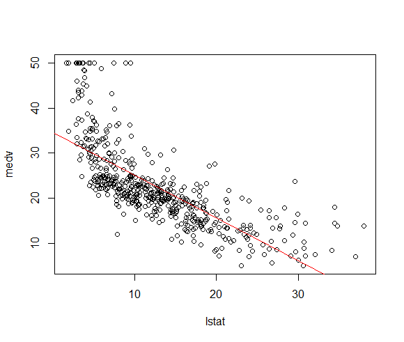
> #测试数据散点图
> plot(lstat,medv)
> #画回归拟合直线
> abline(lm.fit,col='red')
>
> #诊断图
> #图板分区
> par(mfrow=c(2,2))
>
> plot(lm.fit)
>

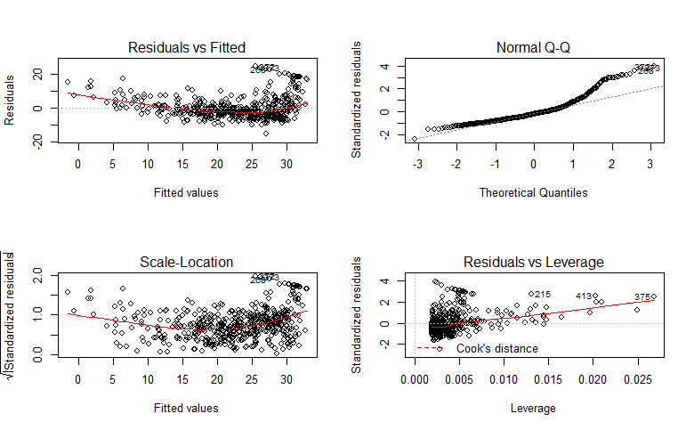
残差图和标准化残差图显示有明显的非线性关系，杠杆图表明第375个样本点是高杠杆点。

---

     多元线性回归

     summary（lm.fit）$r.sq：提取回归方程的决定系数R² ；通过？summary.lm 查看可提取的信息

vif（lm.fit）：查看方差扩大因子（一般回归方程的方差扩大因子大于10的几个变量间存在着多重共线性），需要加载car包。

>
> #多元线性回归
> lm.fit<-lm(medv~lstat+age,data=Boston)
> summary(lm.fit)

Call:
lm(formula = medv ~ lstat + age, data = Boston)

Residuals:
    Min      1Q  Median      3Q     Max
-15.981  -3.978  -1.283   1.968  23.158 

Coefficients:
            Estimate Std. Error t value Pr(>|t|)
(Intercept) 33.22276    0.73085  45.458  < 2e-16 ***
lstat       -1.03207    0.04819 -21.416  < 2e-16 ***
age          0.03454    0.01223   2.826  0.00491 **
---
Signif. codes:  0 ‘***’ 0.001 ‘**’ 0.01 ‘*’ 0.05 ‘.’ 0.1 ‘ ’ 1

Residual standard error: 6.173 on 503 degrees of freedom
Multiple R-squared:  0.5513,	Adjusted R-squared:  0.5495
F-statistic:   309 on 2 and 503 DF,  p-value: < 2.2e-16

>
> lm.summary<-summary(lm.fit)
> #提取R^2
> lm.summary$r.sq
[1] 0.5512689
>
> ##方差扩大因子
> library(car)
> vif(lm.fit)
   lstat      age
1.569395 1.569395
>

---

  非线性

      lm(y~x₁+x₂+x₁:x₂) : x₁:x₂ 只表示x₁^.x₂  ； x1*x2 表示x₁+x₂+x₁^.x₂ ;

lm(y~x+I(x^2)) : 在lm(...)内表示变量的高次项 I(x^2)，直接用x^2是错误的。

>
>
> ##变量间的交互项
>
> lm.fit<-lm(medv~lstat+age+lstat:age,data=Boston)
> summary(lm.fit)

Call:
lm(formula = medv ~ lstat + age + lstat:age, data = Boston)

Residuals:
    Min      1Q  Median      3Q     Max
-15.806  -4.045  -1.333   2.085  27.552 

Coefficients:
              Estimate Std. Error t value Pr(>|t|)
(Intercept) 36.0885359  1.4698355  24.553  < 2e-16 ***
lstat       -1.3921168  0.1674555  -8.313 8.78e-16 ***
age         -0.0007209  0.0198792  -0.036   0.9711
lstat:age    0.0041560  0.0018518   2.244   0.0252 *
---
Signif. codes:  0 ‘***’ 0.001 ‘**’ 0.01 ‘*’ 0.05 ‘.’ 0.1 ‘ ’ 1

Residual standard error: 6.149 on 502 degrees of freedom
Multiple R-squared:  0.5557,	Adjusted R-squared:  0.5531
F-statistic: 209.3 on 3 and 502 DF,  p-value: < 2.2e-16

>
> ##变量的高次项
> lm.fit2<-lm(medv~lstat+I(lstat^2))
> summary(lm.fit2)

Call:
lm(formula = medv ~ lstat + I(lstat^2))

Residuals:
     Min       1Q   Median       3Q      Max
-15.2834  -3.8313  -0.5295   2.3095  25.4148 

Coefficients:
             Estimate Std. Error t value Pr(>|t|)
(Intercept) 42.862007   0.872084   49.15   <2e-16 ***
lstat       -2.332821   0.123803  -18.84   <2e-16 ***
I(lstat^2)   0.043547   0.003745   11.63   <2e-16 ***
---
Signif. codes:  0 ‘***’ 0.001 ‘**’ 0.01 ‘*’ 0.05 ‘.’ 0.1 ‘ ’ 1

Residual standard error: 5.524 on 503 degrees of freedom
Multiple R-squared:  0.6407,	Adjusted R-squared:  0.6393
F-statistic: 448.5 on 2 and 503 DF,  p-value: < 2.2e-16

>
> ##方差分析
> lm.fit1<-lm(medv~lstat)
>
> anova(lm.fit1,lm.fit2)
Analysis of Variance Table

Model 1: medv ~ lstat
Model 2: medv ~ lstat + I(lstat^2)
  Res.Df   RSS Df Sum of Sq     F    Pr(>F)
1    504 19472
2    503 15347  1    4125.1 135.2 < 2.2e-16 ***
---
Signif. codes:  0 ‘***’ 0.001 ‘**’ 0.01 ‘*’ 0.05 ‘.’ 0.1 ‘ ’ 1
>
>

---

定性变量

contrasts(...) : 查看及设置虚拟变量

>
> head(Carseats)
  Sales CompPrice Income Advertising Population Price ShelveLoc Age Education Urban  US
1  9.50       138     73          11        276   120       Bad  42        17   Yes Yes
2 11.22       111     48          16        260    83      Good  65        10   Yes Yes
3 10.06       113     35          10        269    80    Medium  59        12   Yes Yes
4  7.40       117    100           4        466    97    Medium  55        14   Yes Yes
5  4.15       141     64           3        340   128       Bad  38        13   Yes  No
6 10.81       124    113          13        501    72       Bad  78        16    No Yes
>
> lm.fit<-lm(Sales~CompPrice+Income+ShelveLoc,data=Carseats)
> summary(lm.fit)

Call:
lm(formula = Sales ~ CompPrice + Income + ShelveLoc, data = Carseats)

Residuals:
    Min      1Q  Median      3Q     Max
-7.5611 -1.6096 -0.1409  1.6263  6.1845 

Coefficients:
                Estimate Std. Error t value Pr(>|t|)
(Intercept)     2.875874   1.023857   2.809  0.00522 **
CompPrice       0.010634   0.007489   1.420  0.15638
Income          0.018388   0.004111   4.473 1.01e-05 ***
ShelveLocGood   4.750942   0.340955  13.934  < 2e-16 ***
ShelveLocMedium 1.861994   0.280481   6.639 1.05e-10 ***
---
Signif. codes:  0 ‘***’ 0.001 ‘**’ 0.01 ‘*’ 0.05 ‘.’ 0.1 ‘ ’ 1

Residual standard error: 2.285 on 395 degrees of freedom
Multiple R-squared:  0.3519,	Adjusted R-squared:  0.3454
F-statistic: 53.63 on 4 and 395 DF,  p-value: < 2.2e-16

>
> ##查看虚拟变量
> contrasts(Carseats$ShelveLoc)
       Good Medium
Bad       0      0
Good      1      0
Medium    0      1
>