Notes on Probabilistic Latent Semantic Analysis (PLSA)

转自：http://www.hongliangjie.com/2010/01/04/notes-on-probabilistic-latent-semantic-analysis-plsa/

I highly recommend you read the more detailed version of http://arxiv.org/abs/1212.3900

Formulation of PLSA

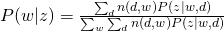
There are two ways to formulate PLSA. They are equivalent but may lead to different inference process.

1. 
2. 

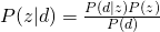
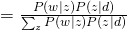
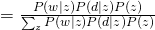
Let’s see why these two equations are equivalent by using Bayes rule.

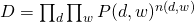
The whole data set is generated as (we assume that all words are generated independently):

The Log-likelihood of the whole data set for (1) and (2) are:

EM

For or , the optimization is hard due to the log of sum. Therefore, an algorithm called Expectation-Maximization is usually employed. Before we introduce anything about EM, please note that EM is only guarantee to find a local optimum (although it may be a global one).

First, we see how EM works in general. As we shown for PLSA, we usually want to estimate the likelihood of data, namely , given the paramter . The easiest way is to obtain a maximum likelihood estimator by maximizing . However, sometimes, we also want to include some hidden variables which are usually useful for our task. Therefore, what we really want to maximize is , the complete likelihood. Now, our attention becomes to this complete likelihood. Again, directly maximizing this likelihood is usually difficult. What we would like to show here is to obtain a lower bound of the likelihood and maximize this lower bound.

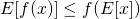
We need Jensen’s Inequality to help us obtain this lower bound. For any convex function , Jensen’s Inequality states that :

Thus, it is not difficult to show that :

and for concave functions (like logarithm), it is :

Back to our complete likelihood, we can obtain the following conclusion by using concave version of Jensen’s Inequality :

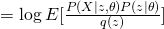
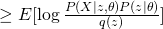
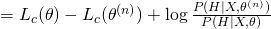
Therefore, we obtained a lower bound of complete likelihood and we want to maximize it as tight as possible. EM is an algorithm that maximize this lower bound through a iterative fashion. Usually, EM first would fix current value and maximize and then use the new value to obtain a new guess on , which is essentially a two stage maximization process. The first step can be shown as follows:

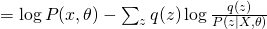
The first term is the same for all . Therefore, in order to maximize the whole equation, we need to minimize KL divergence between and , which eventually leads to the optimum solution of . So, usually for E-step, we use current guess of to calculate the posterior distribution of hidden variable as the new update score. For M-step, it is problem-dependent. We will see how to do that in later discussions.

Another explanation of EM is in terms of optimizing a so-called Q function. We devise the data generation process as . Therefore, the complete likelihood is modified as:

Think about how to maximize . Instead of directly maximizing it, we can iteratively maximize as :

Now take the expectation of this equation, we have:

The last term is always non-negative since it can be recognized as the KL-divergence of and . Therefore, we obtain a lower bound of Likelihood :

The last two terms can be treated as constants as they do not contain the variable , so the lower bound is essentially the first term, which is also sometimes called as “Q-function”.

EM of Formulation 1

In case of Formulation 1, let us introduce hidden variables to indicate which hidden topic is selected to generated in (). Therefore, the complete likelihood can be formulated as :

From the equation above, we can write our Q-function for the complete likelihood :

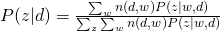
For E-step, simply using Bayes Rule, we can obtain:

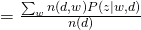
For M-step, we need to maximize Q-function, which needs to be incorporated with other constraints:

and take all derivatives:

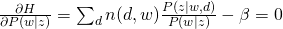
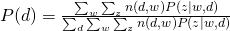
Therefore, we can easily obtain:

EM of Formulation 2

Use similar method to introduce hidden variables to indicate which is selected to generated and and we can have the following complete likelihood :

Therefore, the Q-function would be :

For E-step, again, simply using Bayes Rule, we can obtain:

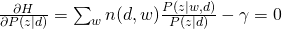
For M-step, we maximize the constraint version of Q-function:

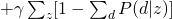
and take all derivatives:

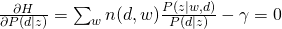
Therefore, we can easily obtain: