ICP（迭代最近点）算法

　　图像配准是图像处理研究领域中的一个典型问题和技术难点，其目的在于比较或融合针对同一对象在不同条件下获取的图像，例如图像会来自不同的采集设备，取自不同的时间，不同的拍摄视角等等，有时也需要用到针对不同对象的图像配准问题。具体地说，对于一组图像数据集中的两幅图像，通过寻找一种空间变换把一幅图像映射到另一幅图像，使得两图中对应于空间同一位置的点一一对应起来，从而达到信息融合的目的。 一个经典的应用是场景的重建，比如说一张茶几上摆了很多杯具，用深度摄像机进行场景的扫描，通常不可能通过一次采集就将场景中的物体全部扫描完成，只能是获取场景不同角度的点云，然后将这些点云融合在一起，获得一个完整的场景。

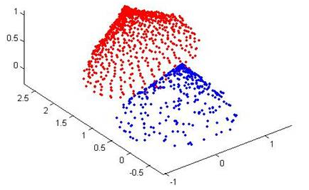
　　ICP（Iterative Closest Point迭代最近点）算法是一种点集对点集配准方法。如下图所示，PR（红色点云）和RB（蓝色点云）是两个点集，该算法就是计算怎么把PB平移旋转，使PB和PR尽量重叠。

　　用数学语言描述如下，即ICP算法的实质是基于最小二乘法的最优匹配，它重复进行“确定对应关系的点集→计算最优刚体变换”的过程，直到某个表示正确匹配的收敛准则得到满足。

ICP算法基本思想：

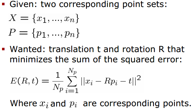
　　如果知道正确的点对应，那么两个点集之间的相对变换（旋转、平移）就可以求得封闭解。

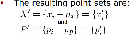
　　首先计算两个点集X和P的质心，分别为μ_x和μ_p

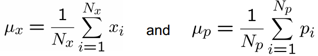
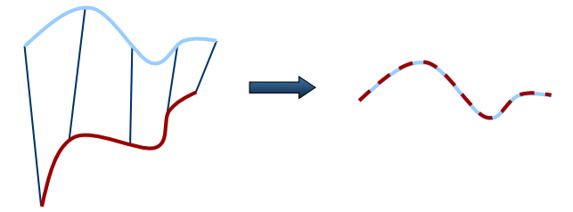
　　然后在两个点集中分别减去对应的质心（Subtract the corresponding center of mass from every point in the two point sets before calculating the transformation）

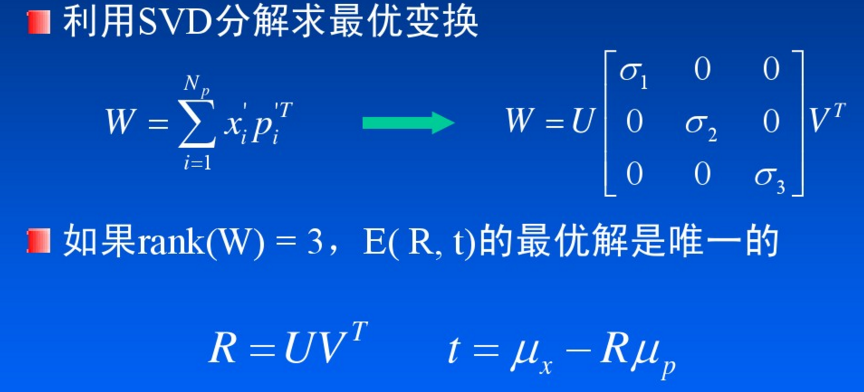
　　目标函数E(R,t)的优化是ICP算法的最后一个阶段。在求得目标函数后，采用什么样的方法来使其收敛到最小，也是一个比较重要的问题。求解方法有基于奇异值分解的方法、四元数方法等。

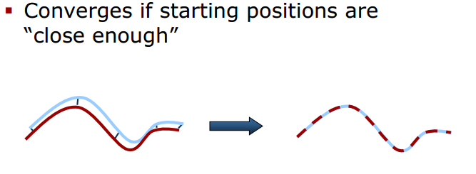
　　如果初始点“足够近”，可以保证收敛性

ICP算法优点：

• 可以获得非常精确的配准效果
• 不必对处理的点集进行分割和特征提取
• 在较好的初值情况下，可以得到很好的算法收敛性

ICP算法的不足之处： 

• 在搜索对应点的过程中，计算量非常大，这是传统ICP算法的瓶颈
• 标准ICP算法中寻找对应点时，认为欧氏距离最近的点就是对应点。这种假设有不合理之处，会产生一定数量的错误对应点

　　针对标准ICP算法的不足之处，许多研究者提出ICP算法的各种改进版本，主要涉及如下所示的6个方面。

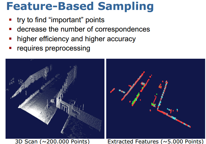
　　标准ICP算法中，选用点集中所有的点来计算对应点，通常用于配准的点集元素数量都是非常巨大的，通过这些点集来计算，所消耗的时间很长。在后来的研究中，提出了各种方法来选择配准元素，这些方法的主要目的都是为了减小点集元素的数目，即如何选用最少的点来表征原始点集的全部特征信息。在点集选取时可以：1.选取所有点；2.均匀采样（Uniform sub-sampling ）；3.随机采样（Random sampling）；4.按特征采样（Feature based Sampling ）；5.法向空间均匀采样（Normal-space sampling），如下图所示，法向采样保证了法向上的连续性（Ensure that samples have normals distributed as uniformly as possible）

　　基于特征的采样使用一些具有明显特征的点集来进行配准，大量减少了对应点的数目。

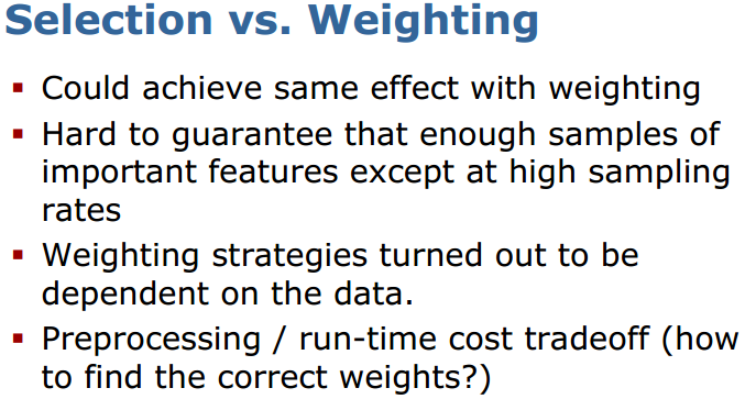
　　点集匹配上有：最近邻点（Closet Point）

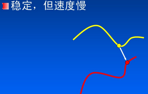　　法方向最近邻点（Normal Shooting）

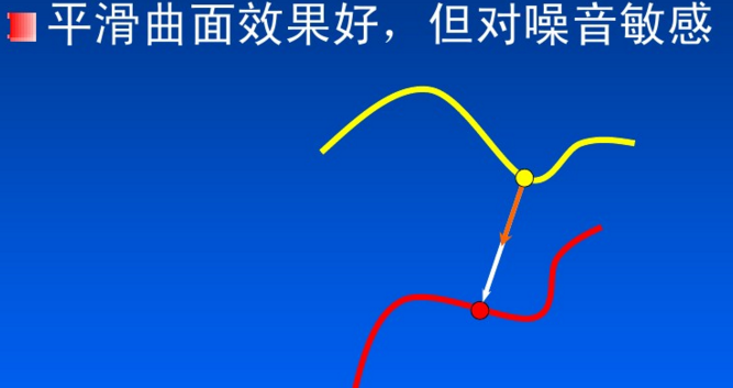
　　投影法（Projection）

　　根据之前算法的描述，下面使用Python来实现基本的ICP算法（代码参考了这里）：

import numpy as np

def best_fit_transform(A, B):
    '''
    Calculates the least-squares best-fit transform between corresponding 3D points A->B
    Input:
      A: Nx3 numpy array of corresponding 3D points
      B: Nx3 numpy array of corresponding 3D points
    Returns:
      T: 4x4 homogeneous transformation matrix
      R: 3x3 rotation matrix
      t: 3x1 column vector
    '''

    assert len(A) == len(B)

    # translate points to their centroids
    centroid_A = np.mean(A, axis=0)
    centroid_B = np.mean(B, axis=0)
    AA = A - centroid_A
    BB = B - centroid_B

    # rotation matrix
    W = np.dot(BB.T, AA)
    U, s, VT = np.linalg.svd(W)
    R = np.dot(U, VT)

    # special reflection case
    if np.linalg.det(R) < 0:
       VT[2,:] *= -1
       R = np.dot(U, VT)

    # translation
    t = centroid_B.T - np.dot(R,centroid_A.T)

    # homogeneous transformation
    T = np.identity(4)
    T[0:3, 0:3] = R
    T[0:3, 3] = t

    return T, R, t

def nearest_neighbor(src, dst):
    '''
    Find the nearest (Euclidean) neighbor in dst for each point in src
    Input:
        src: Nx3 array of points
        dst: Nx3 array of points
    Output:
        distances: Euclidean distances (errors) of the nearest neighbor
        indecies: dst indecies of the nearest neighbor
    '''

    indecies = np.zeros(src.shape[0], dtype=np.int)
    distances = np.zeros(src.shape[0])
    for i, s in enumerate(src):
        min_dist = np.inf
        for j, d in enumerate(dst):
            dist = np.linalg.norm(s-d)
            if dist < min_dist:
                min_dist = dist
                indecies[i] = j
                distances[i] = dist
    return distances, indecies

def icp(A, B, init_pose=None, max_iterations=50, tolerance=0.001):
    '''
    The Iterative Closest Point method
    Input:
        A: Nx3 numpy array of source 3D points
        B: Nx3 numpy array of destination 3D point
        init_pose: 4x4 homogeneous transformation
        max_iterations: exit algorithm after max_iterations
        tolerance: convergence criteria
    Output:
        T: final homogeneous transformation
        distances: Euclidean distances (errors) of the nearest neighbor
    '''

    # make points homogeneous, copy them so as to maintain the originals
    src = np.ones((4,A.shape[0]))
    dst = np.ones((4,B.shape[0]))
    src[0:3,:] = np.copy(A.T)
    dst[0:3,:] = np.copy(B.T)

    # apply the initial pose estimation
    if init_pose is not None:
        src = np.dot(init_pose, src)

    prev_error = 0

    for i in range(max_iterations):
        # find the nearest neighbours between the current source and destination points
        distances, indices = nearest_neighbor(src[0:3,:].T, dst[0:3,:].T)

        # compute the transformation between the current source and nearest destination points
        T,_,_ = best_fit_transform(src[0:3,:].T, dst[0:3,indices].T)

        # update the current source
    # refer to "Introduction to Robotics" Chapter2 P28. Spatial description and transformations
        src = np.dot(T, src)

        # check error
        mean_error = np.sum(distances) / distances.size
        if abs(prev_error-mean_error) < tolerance:
            break
        prev_error = mean_error

    # calculcate final tranformation
    T,_,_ = best_fit_transform(A, src[0:3,:].T)

    return T, distances

if __name__ == "__main__":
    A = np.random.randint(0,101,(20,3))    # 20 points for test

    rotz = lambda theta: np.array([[np.cos(theta),-np.sin(theta),0],
                                       [np.sin(theta),np.cos(theta),0],
                                       [0,0,1]])
    trans = np.array([2.12,-0.2,1.3])
    B = A.dot(rotz(np.pi/4).T) + trans

    T, distances = icp(A, B)

    np.set_printoptions(precision=3,suppress=True)
    print T

　　上面代码创建一个源点集A（在0-100的整数范围内随机生成20个3维数据点），然后将A绕Z轴旋转45°并沿XYZ轴分别移动一小段距离，得到点集B。结果如下，可以看出ICP算法正确的计算出了变换矩阵。

需要注意几点：

　1.首先需要明确公式里的变换是T（P→X）， 即通过旋转和平移把点集P变换到X。我们这里求的变换是T（A→B），要搞清楚对应关系。

　2.本例只用了20个点进行测试，ICP算法在求最近邻点的过程中需要计算20×20次距离并比较大小。如果点的数目巨大，那算法的效率将非常低。

　3.两个点集的初始相对位置对算法的收敛性有一定影响，最好在“足够近”的条件下进行ICP配准。

　　　　　　　　

参考：

Iterative Closest Point (ICP) and other matching algorithms

http://www.mrpt.org/Iterative_Closest_Point_%28ICP%29_and_other_matching_algorithms

PCL学习笔记二：Registration (ICP算法)

http://www.voidcn.com/blog/u010696366/article/p-3712120.html

https://github.com/ClayFlannigan/icp/blob/master/icp.py

ICP迭代最近点算法综述

http://wenku.baidu.com/link?url=iJJoFALkKpgMl7ilivLCM3teN5yn60TKt5uWM6hIZejYPob8Rcy1R4Tm_2ZyX_DvX_Su9XBFCfPc4TqHioU0Gb93jKbhoj-TQ70vfn4VEJC