机器学习（六）：回归分析——鸢尾花多变量回归、逻辑回归三分类只用numpy，sigmoid、实现RANSAC 线性拟合

[实验1 回归分析]

一、 预备知识

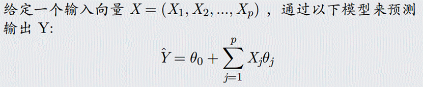
1. 使用梯度下降法求解多变量回归问题

1. 数据集

Iris 鸢尾花数据集是一个经典数据集，在统计学习和机器学习领域都经常被用作示例。数据集内包含 3 类共 150 条记录，每类各 50 个数据，每条记录都有 4 项特征：花萼长度、花萼宽度、花瓣长度、花瓣宽度，可以通过这4个特征预测鸢尾花卉属于（iris-setosa, iris-versicolour, iris-virginica）中的哪一品种。

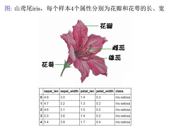
sepal length:花萼长度，单位cm；sepal width:花萼宽度，单位cm

petal length:花瓣长度，单位cm；petal width:花瓣宽度，单位cm

种类:setosa(山鸢尾)，versicolor(杂色鸢尾)，virginica(弗吉尼亚鸢尾)

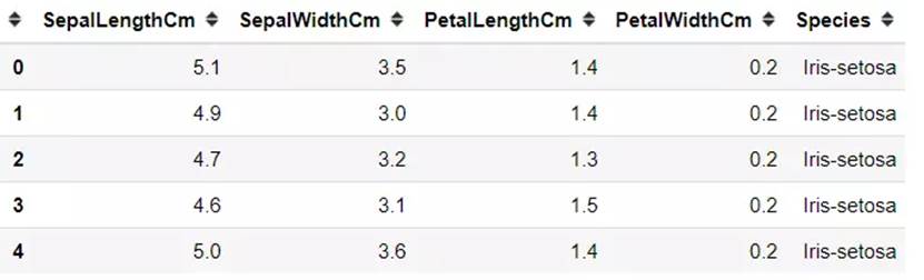
我们用100组数据作为训练数据iris-train.txt，50组数据作为测试数据iris-test.txt。

'setosa' 'versicolor' 'virginica'

0 1 2

二、 实验目的

1. 掌握梯度下降法的原理及设计；

2. 掌握利用梯度下降法解决回归类问题。

三、 实验内容

数据读取：（前4列是特征x，第5列是标签y）

import numpy as np
train_data  = np.loadtxt('iris-train.txt', delimiter='\t')
x_train=np.array(train_data[:,:4])
y_train=np.array(train_data[:,4])

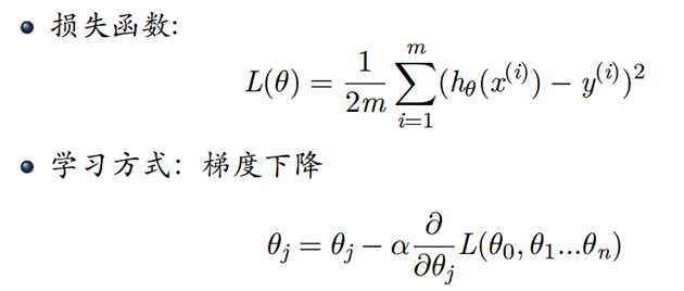
1. 设计多变量回归分析方法，利用训练数据iris-train.txt求解参数

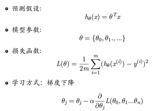
思路：首先确定h（x）函数，由于是4个特征，我们可以取5个参数

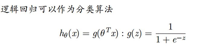
1. 设计逻辑回归分析方法，利用训练数据iris-train.txt求解参数

思路：首先确定h（x）函数，由于是4个特征，我们可以取5个参数

1. 利用测试数据iris-test.txt，统计逻辑回归对测试数据的识别正确率 ACC，Precision，Recall。

四、 操作方法和实验步骤

​ 1.对于多变量回归分析：

\[\alpha \frac{\partial}{\partial \theta _j}L(\theta _0,\theta _1...\theta _n)=\frac { \alpha } { m } X^T(X\theta-y)
\]

​ （1）实现损失函数、h(x)、梯度下降函数等：

def hypothesis(X, theta):
    return np.dot(X, theta)

def cost_function(X, y, theta):
    m = len(y)
    J = np.sum((hypothesis(X, theta) - y) ** 2) / (2 * m)
    return J

def gradient_descent(X, y, theta, alpha, num_iters):
    m = len(y)
    J_history = np.zeros(num_iters)
    for i in range(num_iters):
        theta = theta - (alpha / m) * np.dot(X.T, (hypothesis(X, theta) - y))
        J_history[i] = cost_function(X, y, theta)
    return theta, J_history

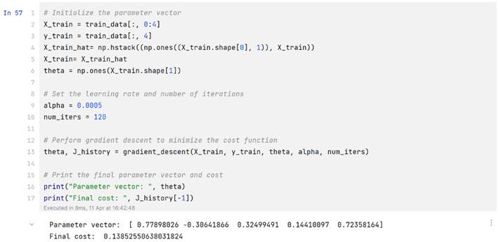
​ （2）处理输出X并开始计算

X_train_hat= np.hstack((np.ones((X_train.shape[0], 1)), X_train))
X_train= X_train_hat
theta = np.ones(X_train.shape[1])

alpha = 0.0005
num_iters = 120

theta, J_history = gradient_descent(X_train, y_train, theta, alpha, num_iters)

print("Parameter vector: ", theta)
print("Final cost: ", J_history[-1])

1. 对于逻辑回归分析

import numpy as np
from sklearn.metrics import classification_report
from sklearn.preprocessing import LabelEncoder

train_data = np.loadtxt("iris/iris-train.txt", delimiter="\t")
X_train = train_data[:, 0:4]
y_train = train_data[:, 4]
encoder = LabelEncoder()
y_train = encoder.fit_transform(y_train)  # Convert class labels to 0, 1, 2
X_train_hat = np.hstack((np.ones((X_train.shape[0], 1)), X_train))
X_train = X_train_hat
def sigmoid(z):
    return 1 / (1 + np.exp(-z))

def cost_function(X, y, theta):
    m = len(y)
    epsilon = 1e-5
    h = sigmoid(np.dot(X, theta))
    J = (-1 / m) * np.sum(y * np.log(h+epsilon) + (1 - y) * np.log(1 - h+epsilon))
    grad = (1 / m) * np.dot(X.T, (h - y))
    return J, grad

def gradient_descent(X, y, theta, alpha, num_iters):
    m = len(y)
    J_history = np.zeros(num_iters)
    for i in range(num_iters):
        J, grad = cost_function(X, y, theta)
        theta = theta - (alpha * grad)
        J_history[i] = J
    return theta, J_history
def logistic_regression(X, y, alpha, num_iters):
    theta = np.ones((X_train.shape[1], 3))
    # Perform gradient descent to minimize the cost function for each class
    for i in range(3):
        y_train_i = (y_train == i).astype(int)
        theta_i, J_history_i = gradient_descent(X_train, y_train_i, theta[:, i], alpha, num_iters)
        import matplotlib.pyplot as plt

        plt.plot(J_history_i)
        plt.xlabel('Iterations')
        plt.ylabel('Cost')
        plt.title('Cost function'+str(i))
        plt.show()
        theta[:, i] = theta_i
        print(f"Class {i} parameter vector: {theta_i}")
        print(f"Class {i} final cost: {J_history_i[-1]}")
    return theta
def predict(test_data, theta):
    X_test = test_data[:, 0:4]
    X_test_hat = np.hstack((np.ones((X_test.shape[0], 1)), X_test))
    X_test = X_test_hat
y_test = test_data[:, 4]
    y_test = encoder.transform(y_test)  # Convert class labels to 0, 1, 2
    y_pred = np.zeros(X_test.shape[0])
    for i in range(3):
        sigmoid_outputs = sigmoid(np.dot(X_test, theta[:, i]))
        threshold = np.median(sigmoid_outputs[y_test == i])#不采用统一的阈值，而是采用每个类别的中位数作为阈值
        y_pred_i = (sigmoid_outputs >= threshold).astype(int)
        y_pred[y_pred_i == 1] = i
    y_pred = encoder.inverse_transform(y_pred.astype(int))  # Convert class labels back to original values
    print(classification_report(y_test, y_pred))

test_data = np.loadtxt("iris/iris-test.txt", delimiter="\t")
theta = logistic_regression(X_train, y_train, 0.0005, 5000)
predict(test_data, theta)

实验结果和分析

1.对于多变量回归分析的实验结果：

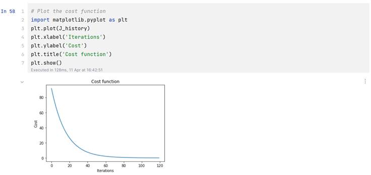
代价曲线：

那么计算函数也就是：

\[y=-0.306x_1+0.0653x_2+0.280x_3+0.697x_4-0.713
\]

​ 2.对于逻辑回归分析的实验结果

代价曲线：

​

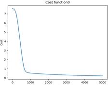
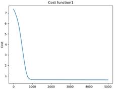
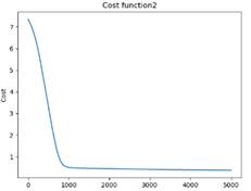
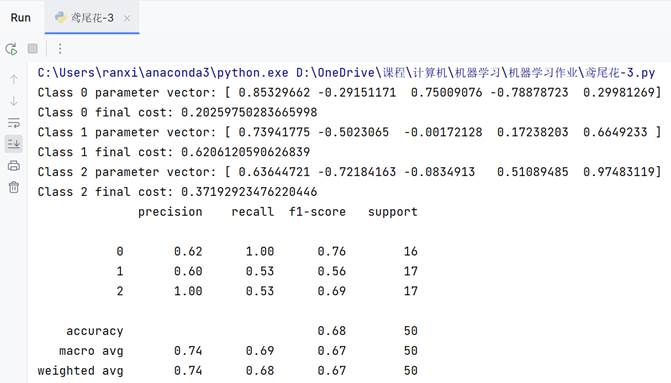
​ 利用测试数据iris-test.txt，统计逻辑回归对测试数据的识别正确率 ACC，Precision，Recall：

​ 通过sigmoid函数实现的逻辑回归只能处理二分类，我是通过分别计算三个二分类实现的。【猜测：预测1时把0和2归为同一类会对模型产生误导】

​ 由于实现方法是One VS One.效果并不是很好，而且得到如下结果还是在处理sigmoid函数结果时还修改了原本0.5的阈值，有泄露结果的嫌疑。

（不采用统一的阈值，而是采用每个类别的h函数结果中位数作为阈值）

五、 思考题

给出 RANSAC 线性拟合的 python 实现

import random
import numpy as np
from matplotlib import pyplot as plt

def ransac_line_fit(data, n_iterations, threshold):
    """
    RANSAC algorithm for linear regression.

    Parameters:
    data (list): list of tuples representing the data points
    n_iterations (int): number of iterations to run RANSAC
    threshold (float): maximum distance a point can be from the line to be considered an inlier

    Returns:
    tuple: slope and y-intercept of the best fit line
    """
    best_slope, best_intercept = None, None
    best_inliers = []

    for i in range(n_iterations):
        # Randomly select two points from the data
        sample = random.sample(data, 2)
        x1, y1 = sample[0]
        x2, y2 = sample[1]

        # Calculate slope and y-intercept of line connecting the two points
        slope = (y2 - y1) / (x2 - x1)
        intercept = y1 - slope * x1

        # Find inliers within threshold distance of the line
        inliers = []
        outliers = []
        for point in data:
            x, y = point
            distance = abs(y - (slope * x + intercept))
            distance = distance / np.sqrt(slope ** 2 + 1)
            if distance <= threshold:
                inliers.append(point)
            else:
                outliers.append(point)

        # If the number of inliers is greater than the current best, update the best fit line
        if len(inliers) > len(best_inliers):
            best_slope = slope
            best_intercept = intercept
            best_inliers = inliers

    outliers = [point for point in data if point not in best_inliers]
    # Plot the data points, best fit line, and inliers and outliers
    fig, ax = plt.subplots()
    # ax.scatter([x for x, y in data], [y for x, y in data], color='black')
    ax.scatter([x for x, y in best_inliers], [y for x, y in best_inliers], color='green')
    ax.scatter([x for x, y in outliers], [y for x, y in outliers], color='black')
    x_vals = np.array([-5,5])
    y_vals = best_slope * x_vals + best_intercept
    ax.plot(x_vals, y_vals, '-', color='red')
    # threshold_line = best_slope * x_vals + best_intercept + threshold*np.sqrt((1/best_slope) ** 2 + 1)
    threshold_line = best_slope * x_vals + best_intercept + threshold * np.sqrt(best_slope ** 2 + 1)
    ax.plot(x_vals, threshold_line, '--', color='blue')
    # threshold_line = best_slope * x_vals + best_intercept - threshold*np.sqrt((1/best_slope) ** 2 + 1)
    threshold_line = best_slope * x_vals + best_intercept - threshold * np.sqrt(best_slope ** 2 + 1)
    ax.plot(x_vals, threshold_line, '--', color='blue')
    # ax.set_xlim([-10, 10])
    ax.set_ylim([-6, 6])
    plt.show()

    return best_slope, best_intercept

import numpy as np

# Generate 10 random points with x values between 0 and 10 and y values between -5 and 5
data = [(x, y) for x, y in zip(np.random.uniform(-5, 5, 10), np.random.uniform(-5, 5, 10))]

print(data)

# Fit a line to the data using RANSAC
slope, intercept = ransac_line_fit(data, 10000, 1)
print(slope, intercept)

结果：