深度学习之深L层神经网络

声明

本文参考(8条消息) 【中文】【吴恩达课后编程作业】Course 1 - 神经网络和深度学习 - 第四周作业(1&2)_何宽的博客-CSDN博客

力求自己理解，刚刚走进深度学习希望可以一起探索。

本文所使用的资料已上传到百度网盘【点击下载】，提取码：xx1w，请在开始之前下载好所需资料，并将资料与代码放在相同界面

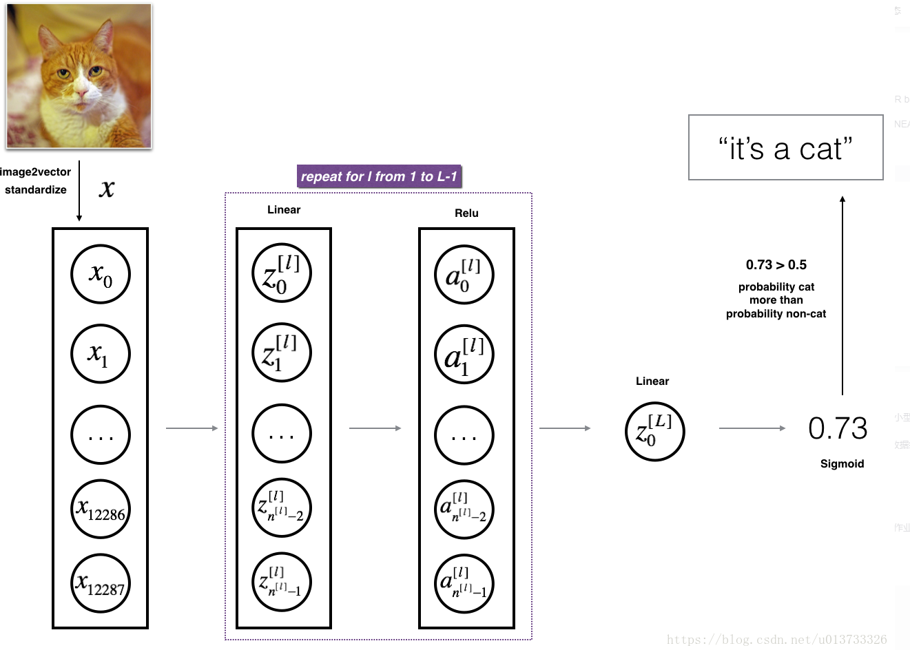
在正式开始之前，我们先来了解一下我们要做什么。在本次教程中，我们要构建两个神经网络，一个是构建两层的神经网络，一个是构建多层的神经网络，多层神经网络的层数可以自己定义。本次的教程的难度有所提升，但是我会力求深入简出。在这里，我们简单的讲一下难点，本文会提到**[LINEAR-> ACTIVATION]转发函数，比如我有一个多层的神经网络，结构是输入层->隐藏层->隐藏层->···->隐藏层->输出层**，在每一层中，我会首先计算Z = np.dot(W,A) + b，这叫做【linear_forward】，然后再计算A = relu(Z) 或者 A = sigmoid(Z)，这叫做【linear_activation_forward】，合并起来就是这一层的计算方法，所以每一层的计算都有两个步骤，先是计算Z，再计算A

流程图

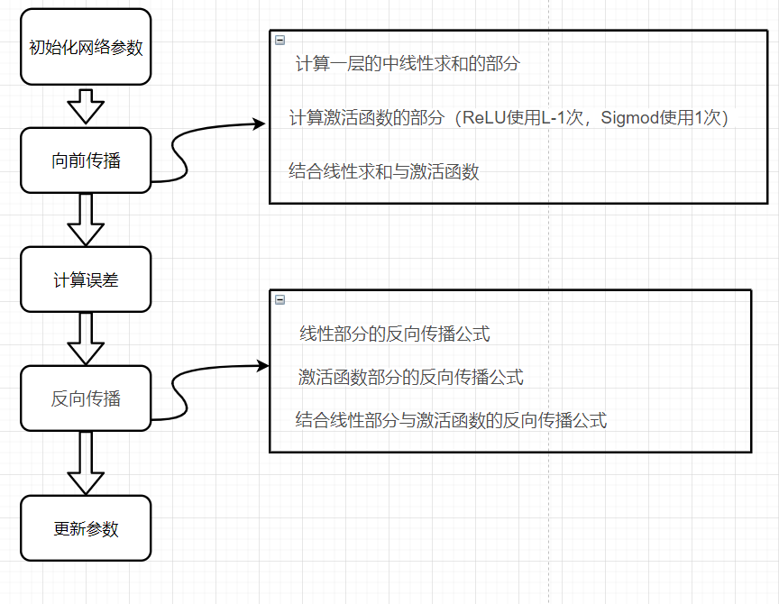
请注意，对于每个前向函数，都有一个相应的后向函数。 这就是为什么在我们的转发模块的每一步都会在cache中存储一些值，cache的值对计算梯度很有用，

在反向传播模块中，我们将使用cache来计算梯度。 现在我们正式开始分别构建两层神经网络和多层神经网络。这里很重要。

import numpy as np
import h5py
import matplotlib.pyplot as plt
import testCases #参见资料包
from dnn_utils import sigmoid, sigmoid_backward, relu, relu_backward #参见资料包
import lr_utils #参见资料包

为了和我的数据匹配，你需要指定随机种子

np.random.seed(1)

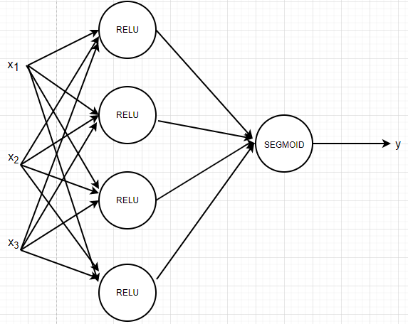
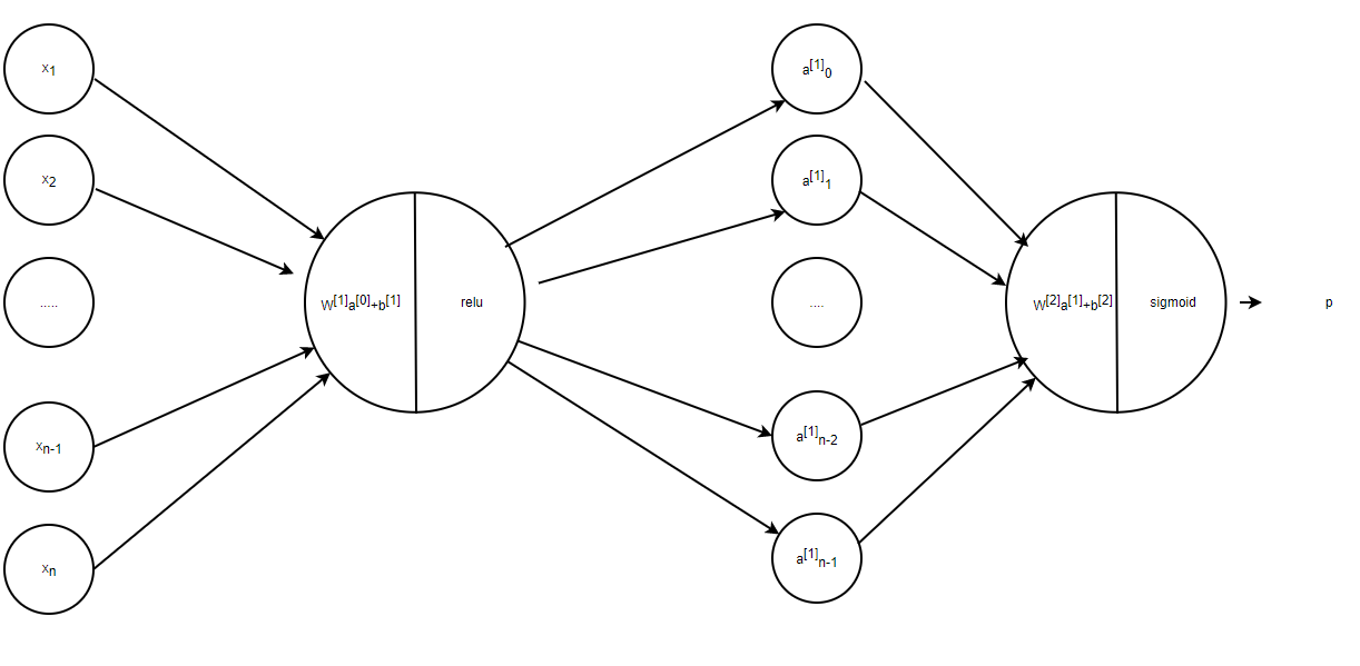
对于一个两层的的神经网络而言，如下图

初始化参数如下

def initialize_parameters(n_x,n_h,n_y):
    """
    此函数是为了初始化两层网络参数而使用的函数。
    参数：
        n_x - 输入层节点数量
        n_h - 隐藏层节点数量
        n_y - 输出层节点数量
 
    返回：
        parameters - 包含你的参数的python字典：
            W1 - 权重矩阵,维度为（n_h，n_x）
            b1 - 偏向量，维度为（n_h，1）
            W2 - 权重矩阵，维度为（n_y，n_h）
            b2 - 偏向量，维度为（n_y，1）
 
    """
    W1 = np.random.randn(n_h, n_x) * 0.01
    b1 = np.zeros((n_h, 1))
    W2 = np.random.randn(n_y, n_h) * 0.01
    b2 = np.zeros((n_y, 1))
 
    #使用断言确保我的数据格式是正确的
    assert(W1.shape == (n_h, n_x))
    assert(b1.shape == (n_h, 1))
    assert(W2.shape == (n_y, n_h))
    assert(b2.shape == (n_y, 1))
 
    parameters = {"W1": W1,
                  "b1": b1,
                  "W2": W2,
                  "b2": b2}
 
    return parameters  

接下来，我们测试一下

print("==============测试initialize_parameters==============")
parameters = initialize_parameters(3,2,1)
print("W1 = " + str(parameters["W1"]))
print("b1 = " + str(parameters["b1"]))
print("W2 = " + str(parameters["W2"]))
print("b2 = " + str(parameters["b2"]))

==============测试initialize_parameters==============
W1 = [[ 0.01624345 -0.00611756 -0.00528172]
 [-0.01072969  0.00865408 -0.02301539]]
b1 = [[0.]
 [0.]]
W2 = [[ 0.01744812 -0.00761207]]
b2 = [[0.]]

两层的神经网络测试已经完毕了，那么对于一个L层的神经网络而言呢？初始化会是什么样的？
当然我们在大学都学过矩阵的乘法和加法吧，我们来看代码

def initialize_parameters_deep(layers_dims):
    """
    此函数是为了初始化多层网络参数而使用的函数。
    参数：
        layers_dims - 包含我们网络中每个图层的节点数量的列表
 
    返回：
        parameters - 包含参数“W1”，“b1”，...，“WL”，“bL”的字典：
                     W1 - 权重矩阵，维度为（layers_dims [1]，layers_dims [1-1]）
                     bl - 偏向量，维度为（layers_dims [1]，1）
    """
    np.random.seed(3)
    parameters = {}
    L = len(layers_dims)
 
    for l in range(1,L):
        parameters["W" + str(l)] = np.random.randn(layers_dims[l], layers_dims[l - 1]) / np.sqrt(layers_dims[l - 1]) # 这个根号其实和上面的0.01是一样目的的
        parameters["b" + str(l)] = np.zeros((layers_dims[l], 1))
 
        #确保我要的数据的格式是正确的
        assert(parameters["W" + str(l)].shape == (layers_dims[l], layers_dims[l-1]))
        assert(parameters["b" + str(l)].shape == (layers_dims[l], 1))
 
    return parameters

我们来测试一下

#测试initialize_parameters_deep
print("==============测试initialize_parameters_deep==============")
layers_dims = [5,4,3]
parameters = initialize_parameters_deep(layers_dims)
print("W1 = " + str(parameters["W1"]))
print("b1 = " + str(parameters["b1"]))
print("W2 = " + str(parameters["W2"]))
print("b2 = " + str(parameters["b2"]))

==============测试initialize_parameters_deep==============
W1 = [[ 0.79989897  0.19521314  0.04315498 -0.83337927 -0.12405178]
 [-0.15865304 -0.03700312 -0.28040323 -0.01959608 -0.21341839]
 [-0.58757818  0.39561516  0.39413741  0.76454432  0.02237573]
 [-0.18097724 -0.24389238 -0.69160568  0.43932807 -0.49241241]]
b1 = [[0.]
 [0.]
 [0.]
 [0.]]
W2 = [[-0.59252326 -0.10282495  0.74307418  0.11835813]
 [-0.51189257 -0.3564966   0.31262248 -0.08025668]
 [-0.38441818 -0.11501536  0.37252813  0.98805539]]
b2 = [[0.]
 [0.]
 [0.]]
我们分别构建了两层和多层神经网络的初始化参数的函数，现在我们开始构建前向传播函数。

---

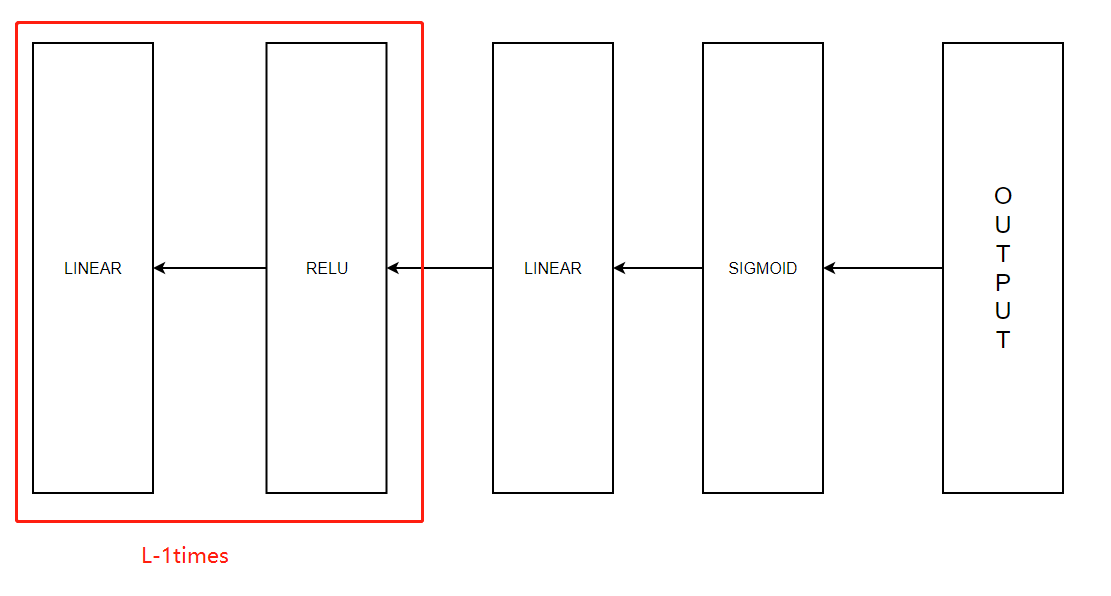
向前传播函数

• LINEAR
• LINEAR - >ACTIVATION，其中激活函数将会使用ReLU或Sigmoid。
• [LINEAR - > RELU] ×（L-1） - > LINEAR - > SIGMOID（整个模型）

线性部分【LINEAR】

前向传播中，线性部分计算如下：

def linear_forward(A,W,b):
    """
    实现前向传播的线性部分。
 
    参数：
        A - 来自上一层（或输入数据）的激活，维度为(上一层的节点数量，示例的数量）
        W - 权重矩阵，numpy数组，维度为（当前图层的节点数量，前一图层的节点数量）
        b - 偏向量，numpy向量，维度为（当前图层节点数量，1）
 
    返回：
         Z - 激活功能的输入，也称为预激活参数
         cache - 一个包含“A”，“W”和“b”的字典，存储这些变量以有效地计算后向传递
    """
    Z = np.dot(W,A) + b
    assert(Z.shape == (W.shape[0],A.shape[1]))
    cache = (A,W,b)
 
    return Z,cache

我们来测试一下：

#测试linear_forward
print("==============测试linear_forward==============")
A,W,b = testCases.linear_forward_test_case()
Z,linear_cache = linear_forward(A,W,b)
print("Z = " + str(Z))

==============测试linear_forward==============
Z = [[ 3.26295337 -1.23429987]]

线性激活部分【LINEAR - >ACTIVATION】

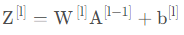
我们为了实现LINEAR->ACTIVATION这个步骤， 使用的公式是：A^[l]=g(z^[l])=g(W^[l]A^[l-1]+b^[l]),其中，函数g会是sigmoid() 或者是 relu()，当然sigmoid()只在输出层使用,现在我们正式构建前向线性激活部分。

我们发现在同一层中A的序列号总是会少1。

def linear_activation_forward(A_prev,W,b,activation):
    """
    实现LINEAR-> ACTIVATION 这一层的前向传播
 
    参数：
        A_prev - 来自上一层（或输入层）的激活，维度为(上一层的节点数量，示例数）
        W - 权重矩阵，numpy数组，维度为（当前层的节点数量，前一层的大小）
        b - 偏向量，numpy阵列，维度为（当前层的节点数量，1）
        activation - 选择在此层中使用的激活函数名，字符串类型，【"sigmoid" | "relu"】
 
    返回：
        A - 激活函数的输出，也称为激活后的值
        cache - 一个包含“linear_cache”和“activation_cache”的字典，我们需要存储它以有效地计算后向传递
    """
 
    if activation == "sigmoid":
        Z, linear_cache = linear_forward(A_prev, W, b)
        A, activation_cache = sigmoid(Z)
    elif activation == "relu":
        Z, linear_cache = linear_forward(A_prev, W, b)
        A, activation_cache = relu(Z)
 
    assert(A.shape == (W.shape[0],A_prev.shape[1]))
    cache = (linear_cache,activation_cache)
 
    return A,cache

我们来测试一下：

#测试linear_activation_forward
print("==============测试linear_activation_forward==============")
A_prev, W,b = testCases.linear_activation_forward_test_case()
 
A, linear_activation_cache = linear_activation_forward(A_prev, W, b, activation = "sigmoid")
print("sigmoid，A = " + str(A))
 
A, linear_activation_cache = linear_activation_forward(A_prev, W, b, activation = "relu")
print("ReLU，A = " + str(A))

==============测试linear_activation_forward==============
sigmoid，A = [[0.96890023 0.11013289]]
ReLU，A = [[3.43896131 0.        ]]

我们把两层模型需要的前向传播函数做完了，那多层网络模型的前向传播是怎样的呢？我们调用上面的那两个函数来实现它，为了在实现L层神经网络时更加方便，

我们需要一个函数来复制前一个函数（带有RELU的linear_activation_forward）L-1次，然后用一个带有SIGMOID的linear_activation_forward跟踪它，

我们来看一下它的结构是怎样的：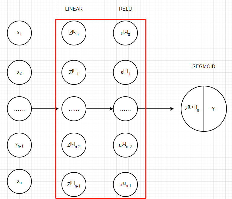

在下面的代码中，AL表示A^[L]=g(Z^[L])=g(W^[L]A^[L-1]+b^[L]),(也可称作 Y_hat)

多层模型的前向传播计算模型代码如下：

def L_model_forward(X,parameters):
    """
    实现[LINEAR-> RELU] *（L-1） - > LINEAR-> SIGMOID计算前向传播，也就是多层网络的前向传播，为后面每一层都执行LINEAR和ACTIVATION
 
    参数：
        X - 数据，numpy数组，维度为（输入节点数量，示例数）
        parameters - initialize_parameters_deep（）的输出
 
    返回：
        AL - 最后的激活值
        caches - 包含以下内容的缓存列表：
                 linear_relu_forward（）的每个cache（有L-1个，索引为从0到L-2）
                 linear_sigmoid_forward（）的cache（只有一个，索引为L-1）
    """
    caches = []
    A = X
    L = len(parameters) // 2  # 因为有两个参数（W,b）因此要整除以2
    for l in range(1,L):
        A_prev = A
        A, cache = linear_activation_forward(A_prev, parameters['W' + str(l)], parameters['b' + str(l)], "relu")
        caches.append(cache)
 
    AL, cache = linear_activation_forward(A, parameters['W' + str(L)], parameters['b' + str(L)], "sigmoid")
    caches.append(cache)
 
    assert(AL.shape == (1,X.shape[1]))
 
    return AL,caches

我们来测试一下：

#测试L_model_forward
print("==============测试L_model_forward==============")
X,parameters = testCases.L_model_forward_test_case()
AL,caches = L_model_forward(X,parameters)
print("AL = " + str(AL))
print("caches 的长度为 = " + str(len(caches)))

==============测试L_model_forward==============
AL = [[0.17007265 0.2524272 ]]
caches 的长度为 = 2

计算成本

我们已经把这两个模型的前向传播部分完成了，我们需要计算成本（误差），以确定它到底有没有在学习，成本的计算公式如：

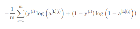
def compute_cost(AL,Y):
    """
    上面定义的成本函数。
 
    参数：
        AL - 与标签预测相对应的概率向量，维度为（1，示例数量）
        Y - 标签向量（例如：如果不是猫，则为0，如果是猫则为1），维度为（1，数量）
 
    返回：
        cost - 交叉熵成本
    """
    m = Y.shape[1]
    cost = -np.sum(np.multiply(np.log(AL),Y) + np.multiply(np.log(1 - AL), 1 - Y)) / m
 
    cost = np.squeeze(cost)
    assert(cost.shape == ())
 
    return cost

我们来测试一下：

#测试compute_cost
print("==============测试compute_cost==============")
Y,AL = testCases.compute_cost_test_case()
print("cost = " + str(compute_cost(AL, Y)))

==============测试compute_cost==============
cost = 0.414931599615397
我们已经把误差值计算出来了，现在开始进行反向传播

---

反向传播

反向传播用于计算相对于参数的损失函数的梯度，我们来看看向前和向后传播的流程图：

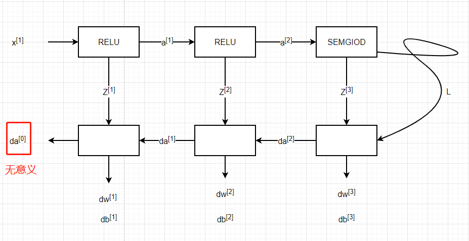
与前向传播类似，我们有需要使用三个步骤来构建反向传播：

LINEAR 后向计算
LINEAR -> ACTIVATION 后向计算，其中ACTIVATION 计算Relu或者Sigmoid 的结果
[LINEAR -> RELU] × \times× (L-1) -> LINEAR -> SIGMOID 后向计算 (整个模型)

线性部分【LINEAR backward】

我们来实现后向传播线性部分：

def linear_backward(dZ,cache):
    """
    为单层实现反向传播的线性部分（第L层）
 
    参数：
         dZ - 相对于（当前第l层的）线性输出的成本梯度
         cache - 来自当前层前向传播的值的元组（A_prev，W，b）
 
    返回：
         dA_prev - 相对于激活（前一层l-1）的成本梯度，与A_prev维度相同
         dW - 相对于W（当前层l）的成本梯度，与W的维度相同
         db - 相对于b（当前层l）的成本梯度，与b维度相同
    """
    A_prev, W, b = cache
    m = A_prev.shape[1]
    dW = np.dot(dZ, A_prev.T) / m
    db = np.sum(dZ, axis=1, keepdims=True) / m
    dA_prev = np.dot(W.T, dZ)
 
    assert (dA_prev.shape == A_prev.shape)
    assert (dW.shape == W.shape)
    assert (db.shape == b.shape)
 
    return dA_prev, dW, db

我们来测试一下：

#测试linear_backward
print("==============测试linear_backward==============")
dZ, linear_cache = testCases.linear_backward_test_case()
 
dA_prev, dW, db = linear_backward(dZ, linear_cache)
print ("dA_prev = "+ str(dA_prev))
print ("dW = " + str(dW))
print ("db = " + str(db))

==============测试linear_backward==============
dA_prev = [[ 0.51822968 -0.19517421]
 [-0.40506361  0.15255393]
 [ 2.37496825 -0.89445391]]
dW = [[-0.10076895  1.40685096  1.64992505]]
db = [[0.50629448]]

线性激活部分【LINEAR -> ACTIVATION backward】

如果 g ( . )  是激活函数, 那么sigmoid_backward 和 relu_backward 这样计算：dZ^[L]=dA^[L]*g(Z^[L])

我们先在正式开始实现后向线性激活：

def linear_activation_backward(dA,cache,activation="relu"):
    """
    实现LINEAR-> ACTIVATION层的后向传播。
 
    参数：
         dA - 当前层l的激活后的梯度值
         cache - 我们存储的用于有效计算反向传播的值的元组（值为linear_cache，activation_cache）
         activation - 要在此层中使用的激活函数名，字符串类型，【"sigmoid" | "relu"】
    返回：
         dA_prev - 相对于激活（前一层l-1）的成本梯度值，与A_prev维度相同
         dW - 相对于W（当前层l）的成本梯度值，与W的维度相同
         db - 相对于b（当前层l）的成本梯度值，与b的维度相同
    """
    linear_cache, activation_cache = cache
    if activation == "relu":
        dZ = relu_backward(dA, activation_cache)
        dA_prev, dW, db = linear_backward(dZ, linear_cache)
    elif activation == "sigmoid":
        dZ = sigmoid_backward(dA, activation_cache)
        dA_prev, dW, db = linear_backward(dZ, linear_cache)
 
    return dA_prev,dW,db

下面我们来测试一下：

#测试linear_activation_backward
print("==============测试linear_activation_backward==============")
AL, linear_activation_cache = testCases.linear_activation_backward_test_case()
 
dA_prev, dW, db = linear_activation_backward(AL, linear_activation_cache, activation = "sigmoid")
print ("sigmoid:")
print ("dA_prev = "+ str(dA_prev))
print ("dW = " + str(dW))
print ("db = " + str(db) + "\n")
 
dA_prev, dW, db = linear_activation_backward(AL, linear_activation_cache, activation = "relu")
print ("relu:")
print ("dA_prev = "+ str(dA_prev))
print ("dW = " + str(dW))
print ("db = " + str(db))

==============测试linear_activation_backward==============
sigmoid:
dA_prev = [[ 0.11017994  0.01105339]
 [ 0.09466817  0.00949723]
 [-0.05743092 -0.00576154]]
dW = [[ 0.10266786  0.09778551 -0.01968084]]
db = [[-0.05729622]]
 
relu:
dA_prev = [[ 0.44090989 -0.        ]
 [ 0.37883606 -0.        ]
 [-0.2298228   0.        ]]
dW = [[ 0.44513824  0.37371418 -0.10478989]]
db = [[-0.20837892]]
我们已经把两层模型的后向计算完成了，对于多层模型我们也需要这两个函数来完成，我们来看一下流程图：

在之前的前向计算中，我们存储了一些包含包含（X，W，b和Z）的cache，我们将会使用它们来计算梯度值，

所以，在L层模型中，我们需要从L层遍历所有的隐藏层，在每一步中，我们需要使用那一层的cache值来进行反向传播。

我们开始构建多层模型向后传播函数：

def L_model_backward(AL,Y,caches):
    """
    对[LINEAR-> RELU] *（L-1） - > LINEAR - > SIGMOID组执行反向传播，就是多层网络的向后传播
 
    参数：
     AL - 概率向量，正向传播的输出（L_model_forward（））
     Y - 标签向量（例如：如果不是猫，则为0，如果是猫则为1），维度为（1，数量）
     caches - 包含以下内容的cache列表：
                 linear_activation_forward（"relu"）的cache，不包含输出层
                 linear_activation_forward（"sigmoid"）的cache
 
    返回：
     grads - 具有梯度值的字典
              grads [“dA”+ str（l）] = ...
              grads [“dW”+ str（l）] = ...
              grads [“db”+ str（l）] = ...
    """
    grads = {}
    L = len(caches)
    m = AL.shape[1]
    Y = Y.reshape(AL.shape)
    dAL = - (np.divide(Y, AL) - np.divide(1 - Y, 1 - AL))
 
    current_cache = caches[L-1]
    grads["dA" + str(L)], grads["dW" + str(L)], grads["db" + str(L)] = linear_activation_backward(dAL, current_cache, "sigmoid")
 
    for l in reversed(range(L-1)):
        current_cache = caches[l]
        dA_prev_temp, dW_temp, db_temp = linear_activation_backward(grads["dA" + str(l+2)], current_cache, "relu")
        grads["dA" + str(l + 1)] = dA_prev_temp
        grads["dW" + str(l + 1)] = dW_temp
        grads["db" + str(l + 1)] = db_temp
 
    return grads

相信第一次看到for循环的小伙伴会跟我一样懵，我以我自己的理解来说明：

在同一层a的序号总是比W，b少1；

reversed将列表逆序变成了[L-2,L-3,L-4.....,2,1,0],又因为W没有dw^[0],subsequent全员+1；

千万不要认为str(l+2)是L-2+2=L,列表的顺序依旧是[0,1,2,3,4...],所以str(l+2)是str(0+2)=str(2)

测试一下：

测试L_model_backward
print("==============测试L_model_backward==============")
AL, Y_assess, caches = testCases.L_model_backward_test_case()
grads = L_model_backward(AL, Y_assess, caches)
print ("dW1 = "+ str(grads["dW1"]))
print ("db1 = "+ str(grads["db1"]))
print ("dA0 = "+ str(grads["dA1"]))

==============测试L_model_backward==============
dW1 = [[0.41010002 0.07807203 0.13798444 0.10502167]
 [0.         0.         0.         0.        ]
 [0.05283652 0.01005865 0.01777766 0.0135308 ]]
db1 = [[-0.22007063]
 [ 0.        ]
 [-0.02835349]]
dA0 = [[ 0.12913162 -0.44014127]
 [-0.14175655  0.48317296]
 [ 0.01663708 -0.05670698]]

更新参数

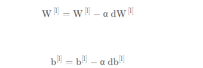
def update_parameters(parameters, grads, learning_rate):
    """
    使用梯度下降更新参数
 
    参数：
     parameters - 包含你的参数的字典
     grads - 包含梯度值的字典，是L_model_backward的输出
 
    返回：
     parameters - 包含更新参数的字典
                   参数[“W”+ str（l）] = ...
                   参数[“b”+ str（l）] = ...
    """
    L = len(parameters) // 2 #整除
    for l in range(L):
        parameters["W" + str(l + 1)] = parameters["W" + str(l + 1)] - learning_rate * grads["dW" + str(l + 1)]
        parameters["b" + str(l + 1)] = parameters["b" + str(l + 1)] - learning_rate * grads["db" + str(l + 1)]
 
    return parameters

测试一下：

#测试update_parameters
print("==============测试update_parameters==============")
parameters, grads = testCases.update_parameters_test_case()
parameters = update_parameters(parameters, grads, 0.1)
 
print ("W1 = "+ str(parameters["W1"]))
print ("b1 = "+ str(parameters["b1"]))
print ("W2 = "+ str(parameters["W2"]))
print ("b2 = "+ str(parameters["b2"]))

==============测试update_parameters==============
W1 = [[-0.59562069 -0.09991781 -2.14584584  1.82662008]
 [-1.76569676 -0.80627147  0.51115557 -1.18258802]
 [-1.0535704  -0.86128581  0.68284052  2.20374577]]
b1 = [[-0.04659241]
 [-1.28888275]
 [ 0.53405496]]
W2 = [[-0.55569196  0.0354055   1.32964895]]
b2 = [[-0.84610769]]
至此为止，我们已经实现该神经网络中所有需要的函数。接下来，我们将这些方法组合在一起，构成一个神经网络类，可以方便的使用。

建立两层的神经网络：

我们正式开始构建两层的神经网络:

def two_layer_model(X,Y,layers_dims,learning_rate=0.0075,num_iterations=3000,print_cost=False,isPlot=True):
    """
    实现一个两层的神经网络，【LINEAR->RELU】 -> 【LINEAR->SIGMOID】
    参数：
        X - 输入的数据，维度为(n_x，例子数)
        Y - 标签，向量，0为非猫，1为猫，维度为(1,数量)
        layers_dims - 层数的向量，维度为(n_y,n_h,n_y)
        learning_rate - 学习率
        num_iterations - 迭代的次数
        print_cost - 是否打印成本值，每100次打印一次
        isPlot - 是否绘制出误差值的图谱
    返回:
        parameters - 一个包含W1，b1，W2，b2的字典变量
    """
    np.random.seed(1)
    grads = {}
    costs = []
    (n_x,n_h,n_y) = layers_dims
 
    """
    初始化参数
    """
    parameters = initialize_parameters(n_x, n_h, n_y)
 
    W1 = parameters["W1"]
    b1 = parameters["b1"]
    W2 = parameters["W2"]
    b2 = parameters["b2"]
 
    """
    开始进行迭代
    """
    for i in range(0,num_iterations):
        #前向传播
        A1, cache1 = linear_activation_forward(X, W1, b1, "relu")
        A2, cache2 = linear_activation_forward(A1, W2, b2, "sigmoid")
 
        #计算成本
        cost = compute_cost(A2,Y)
 
        #后向传播
        ##初始化后向传播
        dA2 = - (np.divide(Y, A2) - np.divide(1 - Y, 1 - A2))
 
        ##向后传播，输入：“dA2，cache2，cache1”。 输出：“dA1，dW2，db2;还有dA0（未使用），dW1，db1”。
        dA1, dW2, db2 = linear_activation_backward(dA2, cache2, "sigmoid")
        dA0, dW1, db1 = linear_activation_backward(dA1, cache1, "relu")
 
        ##向后传播完成后的数据保存到grads
        grads["dW1"] = dW1
        grads["db1"] = db1
        grads["dW2"] = dW2
        grads["db2"] = db2
 
        #更新参数
        parameters = update_parameters(parameters,grads,learning_rate)
        W1 = parameters["W1"]
        b1 = parameters["b1"]
        W2 = parameters["W2"]
        b2 = parameters["b2"]
 
        #打印成本值，如果print_cost=False则忽略
        if i % 100 == 0:
            #记录成本
            costs.append(cost)
            #是否打印成本值
            if print_cost:
                print("第", i ,"次迭代，成本值为：" ,np.squeeze(cost))
    #迭代完成，根据条件绘制图
    if isPlot:
        plt.plot(np.squeeze(costs))
        plt.ylabel('cost')
        plt.xlabel('iterations (per tens)')
        plt.title("Learning rate =" + str(learning_rate))
        plt.show()
 
    #返回parameters
    return parameters

train_set_x_orig , train_set_y , test_set_x_orig , test_set_y , classes = lr_utils.load_dataset()
 
train_x_flatten = train_set_x_orig.reshape(train_set_x_orig.shape[0], -1).T
test_x_flatten = test_set_x_orig.reshape(test_set_x_orig.shape[0], -1).T
 
train_x = train_x_flatten / 255
train_y = train_set_y
test_x = test_x_flatten / 255
test_y = test_set_y

数据集加载完成，开始正式训练：

n_x = 12288
n_h = 7
n_y = 1
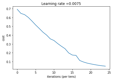
layers_dims = (n_x,n_h,n_y)
 
parameters = two_layer_model(train_x, train_set_y, layers_dims = (n_x, n_h, n_y), num_iterations = 2500, print_cost=True,isPlot=True)

第 0 次迭代，成本值为： 0.6930497356599891
第 100 次迭代，成本值为： 0.6464320953428849
第 200 次迭代，成本值为： 0.6325140647912677
第 300 次迭代，成本值为： 0.6015024920354665
第 400 次迭代，成本值为： 0.5601966311605748
第 500 次迭代，成本值为： 0.515830477276473
第 600 次迭代，成本值为： 0.47549013139433266
第 700 次迭代，成本值为： 0.4339163151225749
第 800 次迭代，成本值为： 0.400797753620389
第 900 次迭代，成本值为： 0.3580705011323798
第 1000 次迭代，成本值为： 0.3394281538366412
第 1100 次迭代，成本值为： 0.30527536361962637
第 1200 次迭代，成本值为： 0.27491377282130186
第 1300 次迭代，成本值为： 0.2468176821061483
第 1400 次迭代，成本值为： 0.19850735037466102
第 1500 次迭代，成本值为： 0.1744831811255663
第 1600 次迭代，成本值为： 0.17080762978097416
第 1700 次迭代，成本值为： 0.11306524562164691
第 1800 次迭代，成本值为： 0.09629426845937152
第 1900 次迭代，成本值为： 0.08342617959726865
第 2000 次迭代，成本值为： 0.07439078704319084
第 2100 次迭代，成本值为： 0.06630748132267936
第 2200 次迭代，成本值为： 0.05919329501038171
第 2300 次迭代，成本值为： 0.05336140348560559
第 2400 次迭代，成本值为： 0.04855478562877018

迭代完成之后我们就可以进行预测了，预测函数如下：

def predict(X, y, parameters):
    """
    该函数用于预测L层神经网络的结果，当然也包含两层
 
    参数：
     X - 测试集
     y - 标签
     parameters - 训练模型的参数
 
    返回：
     p - 给定数据集X的预测
    """
 
    m = X.shape[1]
    n = len(parameters) // 2 # 神经网络的层数
    p = np.zeros((1,m))
 
    #根据参数前向传播
    probas, caches = L_model_forward(X, parameters)
 
    for i in range(0, probas.shape[1]):
        if probas[0,i] > 0.5:
            p[0,i] = 1
        else:
            p[0,i] = 0
 
    print("准确度为: "  + str(float(np.sum((p == y))/m)))
 
    return p

预测函数构建好了我们就开始预测，查看训练集和测试集的准确性：

predictions_train = predict(train_x, train_y, parameters) #训练集
predictions_test = predict(test_x, test_y, parameters) #测试集

准确度为: 1.0
准确度为: 0.72

搭建多层神经网络

def L_layer_model(X, Y, layers_dims, learning_rate=0.0075, num_iterations=3000, print_cost=False,isPlot=True):
    """
    实现一个L层神经网络：[LINEAR-> RELU] *（L-1） - > LINEAR-> SIGMOID。
 
    参数：
        X - 输入的数据，维度为(n_x，例子数)
        Y - 标签，向量，0为非猫，1为猫，维度为(1,数量)
        layers_dims - 层数的向量，维度为(n_y,n_h,···,n_h,n_y)
        learning_rate - 学习率
        num_iterations - 迭代的次数
        print_cost - 是否打印成本值，每100次打印一次
        isPlot - 是否绘制出误差值的图谱
 
    返回：
     parameters - 模型学习的参数。 然后他们可以用来预测。
    """
    np.random.seed(1)
    costs = []
 
    parameters = initialize_parameters_deep(layers_dims)
 
    for i in range(0,num_iterations):
        AL , caches = L_model_forward(X,parameters)
 
        cost = compute_cost(AL,Y)
 
        grads = L_model_backward(AL,Y,caches)
 
        parameters = update_parameters(parameters,grads,learning_rate)
 
        #打印成本值，如果print_cost=False则忽略
        if i % 100 == 0:
            #记录成本
            costs.append(cost)
            #是否打印成本值
            if print_cost:
                print("第", i ,"次迭代，成本值为：" ,np.squeeze(cost))
    #迭代完成，根据条件绘制图
    if isPlot:
        plt.plot(np.squeeze(costs))
        plt.ylabel('cost')
        plt.xlabel('iterations (per tens)')
        plt.title("Learning rate =" + str(learning_rate))
        plt.show()
    return parameters

我们现在开始加载数据集：

train_set_x_orig , train_set_y , test_set_x_orig , test_set_y , classes = lr_utils.load_dataset()
 
train_x_flatten = train_set_x_orig.reshape(train_set_x_orig.shape[0], -1).T
test_x_flatten = test_set_x_orig.reshape(test_set_x_orig.shape[0], -1).T
 
train_x = train_x_flatten / 255
train_y = train_set_y
test_x = test_x_flatten / 255
test_y = test_set_y

数据集加载完成，开始正式训练：

layers_dims = [12288, 20, 7, 5, 1] #  5-layer model
parameters = L_layer_model(train_x, train_y, layers_dims, num_iterations = 2500, print_cost = True,isPlot=True)

第 0 次迭代，成本值为： 0.715731513413713
第 100 次迭代，成本值为： 0.6747377593469114
第 200 次迭代，成本值为： 0.6603365433622127
第 300 次迭代，成本值为： 0.6462887802148751
第 400 次迭代，成本值为： 0.6298131216927773
第 500 次迭代，成本值为： 0.6060056229265339
第 600 次迭代，成本值为： 0.5690041263975134
第 700 次迭代，成本值为： 0.5197965350438059
第 800 次迭代，成本值为： 0.46415716786282285
第 900 次迭代，成本值为： 0.40842030048298916
第 1000 次迭代，成本值为： 0.37315499216069037
第 1100 次迭代，成本值为： 0.30572374573047123
第 1200 次迭代，成本值为： 0.2681015284774084
第 1300 次迭代，成本值为： 0.23872474827672574
第 1400 次迭代，成本值为： 0.20632263257914704
第 1500 次迭代，成本值为： 0.17943886927493524
第 1600 次迭代，成本值为： 0.15798735818801113
第 1700 次迭代，成本值为： 0.14240413012273798
第 1800 次迭代，成本值为： 0.1286516599788517
第 1900 次迭代，成本值为： 0.11244314998153365
第 2000 次迭代，成本值为： 0.08505631034962911
第 2100 次迭代，成本值为： 0.05758391198603161
第 2200 次迭代，成本值为： 0.04456753454692599
第 2300 次迭代，成本值为： 0.038082751665970464
第 2400 次迭代，成本值为： 0.034410749018399016

 

训练完成，我们看一下预测：

pred_train = predict(train_x, train_y, parameters) #训练集
pred_test = predict(test_x, test_y, parameters) #测试集

准确度为: 0.9952153110047847
准确度为: 0.78
72%再到78%，可以看到的是准确度在一点点增加，当然，你也可以手动的去调整layers_dims，准确度可能又会提高一些。

分析

def print_mislabeled_images(classes, X, y, p):
    """
    绘制预测和实际不同的图像。
        X - 数据集
        y - 实际的标签
        p - 预测
    """
    a = p + y
    mislabeled_indices = np.asarray(np.where(a == 1))
    plt.rcParams['figure.figsize'] = (40.0, 40.0) # set default size of plots
    num_images = len(mislabeled_indices[0])
    for i in range(num_images):
        index = mislabeled_indices[1][i]
 
        plt.subplot(2, num_images, i + 1)
        plt.imshow(X[:,index].reshape(64,64,3), interpolation='nearest')
        plt.axis('off')
        plt.title("Prediction: " + classes[int(p[0,index])].decode("utf-8") + " \n Class: " + classes[y[0,index]].decode("utf-8"))
 
print_mislabeled_images(classes, test_x, test_y, pred_test)

分析一下我们就可以得知原因了：

模型往往表现欠佳的几种类型的图像包括：

• 猫身体在一个不同的位置
• 猫出现在相似颜色的背景下
• 不同的猫的颜色和品种
• 相机角度
• 图片的亮度
• 比例变化（猫的图像非常大或很小）

相关库代码

lr_utils.py

# lr_utils.py
import numpy as np
import h5py
 
def load_dataset():
    train_dataset = h5py.File('datasets/train_catvnoncat.h5', "r")
    train_set_x_orig = np.array(train_dataset["train_set_x"][:]) # your train set features
    train_set_y_orig = np.array(train_dataset["train_set_y"][:]) # your train set labels
 
    test_dataset = h5py.File('datasets/test_catvnoncat.h5', "r")
    test_set_x_orig = np.array(test_dataset["test_set_x"][:]) # your test set features
    test_set_y_orig = np.array(test_dataset["test_set_y"][:]) # your test set labels
 
    classes = np.array(test_dataset["list_classes"][:]) # the list of classes
 
    train_set_y_orig = train_set_y_orig.reshape((1, train_set_y_orig.shape[0]))
    test_set_y_orig = test_set_y_orig.reshape((1, test_set_y_orig.shape[0]))
 
    return train_set_x_orig, train_set_y_orig, test_set_x_orig, test_set_y_orig, classes

dnn_utils.py

# dnn_utils.py
import numpy as np
 
def sigmoid(Z):
    """
    Implements the sigmoid activation in numpy
 
    Arguments:
    Z -- numpy array of any shape
 
    Returns:
    A -- output of sigmoid(z), same shape as Z
    cache -- returns Z as well, useful during backpropagation
    """
 
    A = 1/(1+np.exp(-Z))
    cache = Z
 
    return A, cache
 
def sigmoid_backward(dA, cache):
    """
    Implement the backward propagation for a single SIGMOID unit.
 
    Arguments:
    dA -- post-activation gradient, of any shape
    cache -- 'Z' where we store for computing backward propagation efficiently
 
    Returns:
    dZ -- Gradient of the cost with respect to Z
    """
 
    Z = cache
 
    s = 1/(1+np.exp(-Z))
    dZ = dA * s * (1-s)
 
    assert (dZ.shape == Z.shape)
 
    return dZ
 
def relu(Z):
    """
    Implement the RELU function.
 
    Arguments:
    Z -- Output of the linear layer, of any shape
 
    Returns:
    A -- Post-activation parameter, of the same shape as Z
    cache -- a python dictionary containing "A" ; stored for computing the backward pass efficiently
    """
 
    A = np.maximum(0,Z)
 
    assert(A.shape == Z.shape)
 
    cache = Z
    return A, cache
 
def relu_backward(dA, cache):
    """
    Implement the backward propagation for a single RELU unit.
 
    Arguments:
    dA -- post-activation gradient, of any shape
    cache -- 'Z' where we store for computing backward propagation efficiently
 
    Returns:
    dZ -- Gradient of the cost with respect to Z
    """
 
    Z = cache
    dZ = np.array(dA, copy=True) # just converting dz to a correct object.
 
    # When z <= 0, you should set dz to 0 as well.
    dZ[Z <= 0] = 0
 
    assert (dZ.shape == Z.shape)
 
    return dZ

testCase.py

#testCase.py
import numpy as np
 
def linear_forward_test_case():
    np.random.seed(1)
    A = np.random.randn(3,2)
    W = np.random.randn(1,3)
    b = np.random.randn(1,1)
 
    return A, W, b
 
def linear_activation_forward_test_case():
    np.random.seed(2)
    A_prev = np.random.randn(3,2)
    W = np.random.randn(1,3)
    b = np.random.randn(1,1)
    return A_prev, W, b
 
def L_model_forward_test_case():
    np.random.seed(1)
    X = np.random.randn(4,2)
    W1 = np.random.randn(3,4)
    b1 = np.random.randn(3,1)
    W2 = np.random.randn(1,3)
    b2 = np.random.randn(1,1)
    parameters = {"W1": W1,
                  "b1": b1,
                  "W2": W2,
                  "b2": b2}
 
    return X, parameters
 
def compute_cost_test_case():
    Y = np.asarray([[1, 1, 1]])
    aL = np.array([[.8,.9,0.4]])
 
    return Y, aL
 
def linear_backward_test_case():
    np.random.seed(1)
    dZ = np.random.randn(1,2)
    A = np.random.randn(3,2)
    W = np.random.randn(1,3)
    b = np.random.randn(1,1)
    linear_cache = (A, W, b)
    return dZ, linear_cache
 
def linear_activation_backward_test_case():
    np.random.seed(2)
    dA = np.random.randn(1,2)
    A = np.random.randn(3,2)
    W = np.random.randn(1,3)
    b = np.random.randn(1,1)
    Z = np.random.randn(1,2)
    linear_cache = (A, W, b)
    activation_cache = Z
    linear_activation_cache = (linear_cache, activation_cache)
 
    return dA, linear_activation_cache
 
def L_model_backward_test_case():
    np.random.seed(3)
    AL = np.random.randn(1, 2)
    Y = np.array([[1, 0]])
 
    A1 = np.random.randn(4,2)
    W1 = np.random.randn(3,4)
    b1 = np.random.randn(3,1)
    Z1 = np.random.randn(3,2)
    linear_cache_activation_1 = ((A1, W1, b1), Z1)
 
    A2 = np.random.randn(3,2)
    W2 = np.random.randn(1,3)
    b2 = np.random.randn(1,1)
    Z2 = np.random.randn(1,2)
    linear_cache_activation_2 = ( (A2, W2, b2), Z2)
 
    caches = (linear_cache_activation_1, linear_cache_activation_2)
 
    return AL, Y, caches
 
def update_parameters_test_case():
    np.random.seed(2)
    W1 = np.random.randn(3,4)
    b1 = np.random.randn(3,1)
    W2 = np.random.randn(1,3)
    b2 = np.random.randn(1,1)
    parameters = {"W1": W1,
                  "b1": b1,
                  "W2": W2,
                  "b2": b2}
    np.random.seed(3)
    dW1 = np.random.randn(3,4)
    db1 = np.random.randn(3,1)
    dW2 = np.random.randn(1,3)
    db2 = np.random.randn(1,1)
    grads = {"dW1": dW1,
             "db1": db1,
             "dW2": dW2,
             "db2": db2}
 
    return parameters, grads