[cnn][julia]Flux实现卷积神经网络cnn预测手写MNIST
julia_Flux
1.导入Flux.jl和其他所需工具包
using Flux, MLDatasets, Statistics

using Flux: onehotbatch, onecold, logitcrossentropy, params

using MLDatasets: MNIST

using Base.Iterators: partition

using Printf, BSON

using Images

using CUDA,LinearAlgebra,Random

CUDA.allowscalar(false)
# 为学习率、batch、epoch和保存文件的路径设置默认值

Base.@kwdef mutable struct TrainArgs

  lr::Float64 = 3e-3

  epochs::Int = 20

  batch_size = 128

end
TrainArgs
训练集测试集
MNIST 60000训练集 10000测试集
train_data= MLDatasets.MNIST(split=:train)
dataset MNIST:

  metadata  =>    Dict{String, Any} with 3 entries

  split     =>    :train

  features  =>    28×28×60000 Array{Float32, 3}

  targets   =>    60000-element Vector{Int64}
test_data= MLDatasets.MNIST(split=:test)
dataset MNIST:

  metadata  =>    Dict{String, Any} with 3 entries

  split     =>    :test

  features  =>    28×28×10000 Array{Float32, 3}

  targets   =>    10000-element Vector{Int64}
train_data.features
28×28×60000 Array{Float32, 3}:

[:, :, 1] =

 0.0  0.0  0.0  0.0  0.0  0.0       …  0.0       0.0       0.0  0.0  0.0

 0.0  0.0  0.0  0.0  0.0  0.0          0.0       0.0       0.0  0.0  0.0

 0.0  0.0  0.0  0.0  0.0  0.0          0.0       0.0       0.0  0.0  0.0

 0.0  0.0  0.0  0.0  0.0  0.0          0.0       0.0       0.0  0.0  0.0

 0.0  0.0  0.0  0.0  0.0  0.0          0.215686  0.533333  0.0  0.0  0.0

 0.0  0.0  0.0  0.0  0.0  0.0       …  0.67451   0.992157  0.0  0.0  0.0

 0.0  0.0  0.0  0.0  0.0  0.0          0.886275  0.992157  0.0  0.0  0.0

 0.0  0.0  0.0  0.0  0.0  0.0          0.992157  0.992157  0.0  0.0  0.0

 0.0  0.0  0.0  0.0  0.0  0.0          0.992157  0.831373  0.0  0.0  0.0

 0.0  0.0  0.0  0.0  0.0  0.0          0.992157  0.529412  0.0  0.0  0.0

 ⋮                        ⋮         ⋱                      ⋮

 0.0  0.0  0.0  0.0  0.0  0.101961     0.0       0.0       0.0  0.0  0.0

 0.0  0.0  0.0  0.0  0.0  0.65098   …  0.0       0.0       0.0  0.0  0.0

 0.0  0.0  0.0  0.0  0.0  1.0          0.0       0.0       0.0  0.0  0.0

 0.0  0.0  0.0  0.0  0.0  0.968627     0.0       0.0       0.0  0.0  0.0

 0.0  0.0  0.0  0.0  0.0  0.498039     0.0       0.0       0.0  0.0  0.0

 0.0  0.0  0.0  0.0  0.0  0.0          0.0       0.0       0.0  0.0  0.0

 0.0  0.0  0.0  0.0  0.0  0.0       …  0.0       0.0       0.0  0.0  0.0

 0.0  0.0  0.0  0.0  0.0  0.0          0.0       0.0       0.0  0.0  0.0

 0.0  0.0  0.0  0.0  0.0  0.0          0.0       0.0       0.0  0.0  0.0

[:, :, 2] =

 0.0  0.0  0.0  0.0  0.0       0.0       …  0.0        0.0  0.0  0.0  0.0

 0.0  0.0  0.0  0.0  0.0       0.0          0.0        0.0  0.0  0.0  0.0

 0.0  0.0  0.0  0.0  0.0       0.0          0.0        0.0  0.0  0.0  0.0

 0.0  0.0  0.0  0.0  0.0       0.0          0.0        0.0  0.0  0.0  0.0

 0.0  0.0  0.0  0.0  0.0       0.0          0.0        0.0  0.0  0.0  0.0

 0.0  0.0  0.0  0.0  0.0       0.0       …  0.0        0.0  0.0  0.0  0.0

 0.0  0.0  0.0  0.0  0.0       0.0          0.0        0.0  0.0  0.0  0.0

 0.0  0.0  0.0  0.0  0.0       0.0          0.0980392  0.0  0.0  0.0  0.0

 0.0  0.0  0.0  0.0  0.0       0.0          0.501961   0.0  0.0  0.0  0.0

 0.0  0.0  0.0  0.0  0.0       0.0          0.988235   0.0  0.0  0.0  0.0

 ⋮                             ⋮         ⋱                  ⋮

 0.0  0.0  0.0  0.0  0.196078  0.929412     0.0        0.0  0.0  0.0  0.0

 0.0  0.0  0.0  0.0  0.0       0.0       …  0.0        0.0  0.0  0.0  0.0

 0.0  0.0  0.0  0.0  0.0       0.0          0.0        0.0  0.0  0.0  0.0

 0.0  0.0  0.0  0.0  0.0       0.0          0.0        0.0  0.0  0.0  0.0

 0.0  0.0  0.0  0.0  0.0       0.0          0.0        0.0  0.0  0.0  0.0

 0.0  0.0  0.0  0.0  0.0       0.0          0.0        0.0  0.0  0.0  0.0

 0.0  0.0  0.0  0.0  0.0       0.0       …  0.0        0.0  0.0  0.0  0.0

 0.0  0.0  0.0  0.0  0.0       0.0          0.0        0.0  0.0  0.0  0.0

 0.0  0.0  0.0  0.0  0.0       0.0          0.0        0.0  0.0  0.0  0.0

[:, :, 3] =

 0.0  0.0  0.0  0.0  0.0  0.0       0.0       …  0.0  0.0  0.0  0.0  0.0  0.0

 0.0  0.0  0.0  0.0  0.0  0.0       0.0          0.0  0.0  0.0  0.0  0.0  0.0

 0.0  0.0  0.0  0.0  0.0  0.0       0.0          0.0  0.0  0.0  0.0  0.0  0.0

 0.0  0.0  0.0  0.0  0.0  0.0       0.0          0.0  0.0  0.0  0.0  0.0  0.0

 0.0  0.0  0.0  0.0  0.0  0.0       0.243137     0.0  0.0  0.0  0.0  0.0  0.0

 0.0  0.0  0.0  0.0  0.0  0.0       0.317647  …  0.0  0.0  0.0  0.0  0.0  0.0

 0.0  0.0  0.0  0.0  0.0  0.0       0.0          0.0  0.0  0.0  0.0  0.0  0.0

 0.0  0.0  0.0  0.0  0.0  0.0       0.0          0.0  0.0  0.0  0.0  0.0  0.0

 0.0  0.0  0.0  0.0  0.0  0.0       0.0          0.0  0.0  0.0  0.0  0.0  0.0

 0.0  0.0  0.0  0.0  0.0  0.0       0.0          0.0  0.0  0.0  0.0  0.0  0.0

 ⋮                        ⋮                   ⋱                 ⋮

 0.0  0.0  0.0  0.0  0.0  0.0       0.0          0.6  0.6  0.6  0.0  0.0  0.0

 0.0  0.0  0.0  0.0  0.0  0.262745  0.470588  …  0.0  0.0  0.0  0.0  0.0  0.0

 0.0  0.0  0.0  0.0  0.0  0.909804  0.705882     0.0  0.0  0.0  0.0  0.0  0.0

 0.0  0.0  0.0  0.0  0.0  0.152941  0.152941     0.0  0.0  0.0  0.0  0.0  0.0

 0.0  0.0  0.0  0.0  0.0  0.0       0.0          0.0  0.0  0.0  0.0  0.0  0.0

 0.0  0.0  0.0  0.0  0.0  0.0       0.0          0.0  0.0  0.0  0.0  0.0  0.0

 0.0  0.0  0.0  0.0  0.0  0.0       0.0       …  0.0  0.0  0.0  0.0  0.0  0.0

 0.0  0.0  0.0  0.0  0.0  0.0       0.0          0.0  0.0  0.0  0.0  0.0  0.0

 0.0  0.0  0.0  0.0  0.0  0.0       0.0          0.0  0.0  0.0  0.0  0.0  0.0

;;; …

[:, :, 59998] =

 0.0  0.0  0.0  0.0  0.0  0.0       …  0.0       0.0       0.0  0.0  0.0

 0.0  0.0  0.0  0.0  0.0  0.0          0.0       0.0       0.0  0.0  0.0

 0.0  0.0  0.0  0.0  0.0  0.0          0.0       0.0       0.0  0.0  0.0

 0.0  0.0  0.0  0.0  0.0  0.0          0.0       0.0       0.0  0.0  0.0

 0.0  0.0  0.0  0.0  0.0  0.0          0.0       0.0       0.0  0.0  0.0

 0.0  0.0  0.0  0.0  0.0  0.0       …  0.45098   0.0       0.0  0.0  0.0

 0.0  0.0  0.0  0.0  0.0  0.0          0.941176  0.0       0.0  0.0  0.0

 0.0  0.0  0.0  0.0  0.0  0.0          0.988235  0.615686  0.0  0.0  0.0

 0.0  0.0  0.0  0.0  0.0  0.0          0.639216  0.992157  0.0  0.0  0.0

 0.0  0.0  0.0  0.0  0.0  0.0          0.576471  0.992157  0.0  0.0  0.0

 ⋮                        ⋮         ⋱                      ⋮

 0.0  0.0  0.0  0.0  0.0  0.376471     0.0       0.0       0.0  0.0  0.0

 0.0  0.0  0.0  0.0  0.0  0.47451   …  0.0       0.0       0.0  0.0  0.0

 0.0  0.0  0.0  0.0  0.0  0.835294     0.0       0.0       0.0  0.0  0.0

 0.0  0.0  0.0  0.0  0.0  1.0          0.0       0.0       0.0  0.0  0.0

 0.0  0.0  0.0  0.0  0.0  1.0          0.0       0.0       0.0  0.0  0.0

 0.0  0.0  0.0  0.0  0.0  0.47451      0.0       0.0       0.0  0.0  0.0

 0.0  0.0  0.0  0.0  0.0  0.0       …  0.0       0.0       0.0  0.0  0.0

 0.0  0.0  0.0  0.0  0.0  0.0          0.0       0.0       0.0  0.0  0.0

 0.0  0.0  0.0  0.0  0.0  0.0          0.0       0.0       0.0  0.0  0.0

[:, :, 59999] =

 0.0  0.0  0.0       0.0       0.0        …  0.0  0.0  0.0  0.0  0.0  0.0

 0.0  0.0  0.0       0.0       0.0           0.0  0.0  0.0  0.0  0.0  0.0

 0.0  0.0  0.0       0.0       0.0           0.0  0.0  0.0  0.0  0.0  0.0

 0.0  0.0  0.0       0.0       0.0           0.0  0.0  0.0  0.0  0.0  0.0

 0.0  0.0  0.0       0.0       0.0           0.0  0.0  0.0  0.0  0.0  0.0

 ⋮                                        ⋱                 ⋮

 0.0  0.0  0.752941  0.988235  0.745098      0.0  0.0  0.0  0.0  0.0  0.0

 0.0  0.0  0.901961  0.756863  0.0352941  …  0.0  0.0  0.0  0.0  0.0  0.0

 0.0  0.0  0.105882  0.105882  0.0           0.0  0.0  0.0  0.0  0.0  0.0

 0.0  0.0  0.0       0.0       0.0           0.0  0.0  0.0  0.0  0.0  0.0

 0.0  0.0  0.0       0.0       0.0           0.0  0.0  0.0  0.0  0.0  0.0

 0.0  0.0  0.0       0.0       0.0           0.0  0.0  0.0  0.0  0.0  0.0

 0.0  0.0  0.0       0.0       0.0        …  0.0  0.0  0.0  0.0  0.0  0.0

 0.0  0.0  0.0       0.0       0.0           0.0  0.0  0.0  0.0  0.0  0.0

 0.0  0.0  0.0       0.0       0.0           0.0  0.0  0.0  0.0  0.0  0.0

[:, :, 60000] =

 0.0  0.0  0.0  0.0  0.0  0.0  …  0.0       0.0       0.0  0.0  0.0

 0.0  0.0  0.0  0.0  0.0  0.0     0.0       0.0       0.0  0.0  0.0

 0.0  0.0  0.0  0.0  0.0  0.0     0.0       0.0       0.0  0.0  0.0

 0.0  0.0  0.0  0.0  0.0  0.0     0.0       0.0       0.0  0.0  0.0

 0.0  0.0  0.0  0.0  0.0  0.0     0.0       0.0       0.0  0.0  0.0

 0.0  0.0  0.0  0.0  0.0  0.0  …  0.0       0.0       0.0  0.0  0.0

 0.0  0.0  0.0  0.0  0.0  0.0     0.101961  0.0       0.0  0.0  0.0

 0.0  0.0  0.0  0.0  0.0  0.0     0.898039  0.286275  0.0  0.0  0.0

 0.0  0.0  0.0  0.0  0.0  0.0     0.976471  0.756863  0.0  0.0  0.0

 0.0  0.0  0.0  0.0  0.0  0.0     0.690196  0.772549  0.0  0.0  0.0

 ⋮                        ⋮    ⋱                      ⋮

 0.0  0.0  0.0  0.0  0.0  0.0     0.0       0.0       0.0  0.0  0.0

 0.0  0.0  0.0  0.0  0.0  0.0  …  0.0       0.0       0.0  0.0  0.0

 0.0  0.0  0.0  0.0  0.0  0.0     0.0       0.0       0.0  0.0  0.0

 0.0  0.0  0.0  0.0  0.0  0.0     0.0       0.0       0.0  0.0  0.0

 0.0  0.0  0.0  0.0  0.0  0.0     0.0       0.0       0.0  0.0  0.0

 0.0  0.0  0.0  0.0  0.0  0.0     0.0       0.0       0.0  0.0  0.0

 0.0  0.0  0.0  0.0  0.0  0.0  …  0.0       0.0       0.0  0.0  0.0

 0.0  0.0  0.0  0.0  0.0  0.0     0.0       0.0       0.0  0.0  0.0

 0.0  0.0  0.0  0.0  0.0  0.0     0.0       0.0       0.0  0.0  0.0
X_train = reshape(train_data.features, 28,28,1,:)

size(X_train)

pic_1 = X_train[:,:,:,1]
28×28×1 Array{Float32, 3}:

[:, :, 1] =

 0.0  0.0  0.0  0.0  0.0  0.0       …  0.0       0.0       0.0  0.0  0.0

 0.0  0.0  0.0  0.0  0.0  0.0          0.0       0.0       0.0  0.0  0.0

 0.0  0.0  0.0  0.0  0.0  0.0          0.0       0.0       0.0  0.0  0.0

 0.0  0.0  0.0  0.0  0.0  0.0          0.0       0.0       0.0  0.0  0.0

 0.0  0.0  0.0  0.0  0.0  0.0          0.215686  0.533333  0.0  0.0  0.0

 0.0  0.0  0.0  0.0  0.0  0.0       …  0.67451   0.992157  0.0  0.0  0.0

 0.0  0.0  0.0  0.0  0.0  0.0          0.886275  0.992157  0.0  0.0  0.0

 0.0  0.0  0.0  0.0  0.0  0.0          0.992157  0.992157  0.0  0.0  0.0

 0.0  0.0  0.0  0.0  0.0  0.0          0.992157  0.831373  0.0  0.0  0.0

 0.0  0.0  0.0  0.0  0.0  0.0          0.992157  0.529412  0.0  0.0  0.0

 ⋮                        ⋮         ⋱                      ⋮

 0.0  0.0  0.0  0.0  0.0  0.101961     0.0       0.0       0.0  0.0  0.0

 0.0  0.0  0.0  0.0  0.0  0.65098   …  0.0       0.0       0.0  0.0  0.0

 0.0  0.0  0.0  0.0  0.0  1.0          0.0       0.0       0.0  0.0  0.0

 0.0  0.0  0.0  0.0  0.0  0.968627     0.0       0.0       0.0  0.0  0.0

 0.0  0.0  0.0  0.0  0.0  0.498039     0.0       0.0       0.0  0.0  0.0

 0.0  0.0  0.0  0.0  0.0  0.0          0.0       0.0       0.0  0.0  0.0

 0.0  0.0  0.0  0.0  0.0  0.0       …  0.0       0.0       0.0  0.0  0.0

 0.0  0.0  0.0  0.0  0.0  0.0          0.0       0.0       0.0  0.0  0.0

 0.0  0.0  0.0  0.0  0.0  0.0          0.0       0.0       0.0  0.0  0.0
img = pic_1[:,:]
28×28 Matrix{Float32}:

 0.0  0.0  0.0  0.0  0.0  0.0       …  0.0       0.0       0.0  0.0  0.0

 0.0  0.0  0.0  0.0  0.0  0.0          0.0       0.0       0.0  0.0  0.0

 0.0  0.0  0.0  0.0  0.0  0.0          0.0       0.0       0.0  0.0  0.0

 0.0  0.0  0.0  0.0  0.0  0.0          0.0       0.0       0.0  0.0  0.0

 0.0  0.0  0.0  0.0  0.0  0.0          0.215686  0.533333  0.0  0.0  0.0

 0.0  0.0  0.0  0.0  0.0  0.0       …  0.67451   0.992157  0.0  0.0  0.0

 0.0  0.0  0.0  0.0  0.0  0.0          0.886275  0.992157  0.0  0.0  0.0

 0.0  0.0  0.0  0.0  0.0  0.0          0.992157  0.992157  0.0  0.0  0.0

 0.0  0.0  0.0  0.0  0.0  0.0          0.992157  0.831373  0.0  0.0  0.0

 0.0  0.0  0.0  0.0  0.0  0.0          0.992157  0.529412  0.0  0.0  0.0

 ⋮                        ⋮         ⋱                      ⋮

 0.0  0.0  0.0  0.0  0.0  0.101961     0.0       0.0       0.0  0.0  0.0

 0.0  0.0  0.0  0.0  0.0  0.65098   …  0.0       0.0       0.0  0.0  0.0

 0.0  0.0  0.0  0.0  0.0  1.0          0.0       0.0       0.0  0.0  0.0

 0.0  0.0  0.0  0.0  0.0  0.968627     0.0       0.0       0.0  0.0  0.0

 0.0  0.0  0.0  0.0  0.0  0.498039     0.0       0.0       0.0  0.0  0.0

 0.0  0.0  0.0  0.0  0.0  0.0          0.0       0.0       0.0  0.0  0.0

 0.0  0.0  0.0  0.0  0.0  0.0       …  0.0       0.0       0.0  0.0  0.0

 0.0  0.0  0.0  0.0  0.0  0.0          0.0       0.0       0.0  0.0  0.0

 0.0  0.0  0.0  0.0  0.0  0.0          0.0       0.0       0.0  0.0  0.0
colorview(Gray,img')

train_data.targets
60000-element Vector{Int64}:

 5

 0

 4

 1

 9

 2

 1

 3

 1

 4

 ⋮

 2

 9

 5

 1

 8

 3

 5

 6

 8
Flux.onehotbatch(train_data.targets, 0:9)
10×60000 OneHotMatrix(::Vector{UInt32}) with eltype Bool:

 ⋅  1  ⋅  ⋅  ⋅  ⋅  ⋅  ⋅  ⋅  ⋅  ⋅  ⋅  ⋅  …  ⋅  ⋅  ⋅  ⋅  ⋅  ⋅  ⋅  ⋅  ⋅  ⋅  ⋅  ⋅

 ⋅  ⋅  ⋅  1  ⋅  ⋅  1  ⋅  1  ⋅  ⋅  ⋅  ⋅     ⋅  ⋅  ⋅  ⋅  ⋅  ⋅  1  ⋅  ⋅  ⋅  ⋅  ⋅

 ⋅  ⋅  ⋅  ⋅  ⋅  1  ⋅  ⋅  ⋅  ⋅  ⋅  ⋅  ⋅     ⋅  ⋅  ⋅  1  ⋅  ⋅  ⋅  ⋅  ⋅  ⋅  ⋅  ⋅

 ⋅  ⋅  ⋅  ⋅  ⋅  ⋅  ⋅  1  ⋅  ⋅  1  ⋅  1     ⋅  ⋅  ⋅  ⋅  ⋅  ⋅  ⋅  ⋅  1  ⋅  ⋅  ⋅

 ⋅  ⋅  1  ⋅  ⋅  ⋅  ⋅  ⋅  ⋅  1  ⋅  ⋅  ⋅     ⋅  ⋅  ⋅  ⋅  ⋅  ⋅  ⋅  ⋅  ⋅  ⋅  ⋅  ⋅

 1  ⋅  ⋅  ⋅  ⋅  ⋅  ⋅  ⋅  ⋅  ⋅  ⋅  1  ⋅  …  ⋅  ⋅  ⋅  ⋅  ⋅  1  ⋅  ⋅  ⋅  1  ⋅  ⋅

 ⋅  ⋅  ⋅  ⋅  ⋅  ⋅  ⋅  ⋅  ⋅  ⋅  ⋅  ⋅  ⋅     ⋅  ⋅  ⋅  ⋅  ⋅  ⋅  ⋅  ⋅  ⋅  ⋅  1  ⋅

 ⋅  ⋅  ⋅  ⋅  ⋅  ⋅  ⋅  ⋅  ⋅  ⋅  ⋅  ⋅  ⋅     1  ⋅  ⋅  ⋅  ⋅  ⋅  ⋅  ⋅  ⋅  ⋅  ⋅  ⋅

 ⋅  ⋅  ⋅  ⋅  ⋅  ⋅  ⋅  ⋅  ⋅  ⋅  ⋅  ⋅  ⋅     ⋅  1  ⋅  ⋅  ⋅  ⋅  ⋅  1  ⋅  ⋅  ⋅  1

 ⋅  ⋅  ⋅  ⋅  1  ⋅  ⋅  ⋅  ⋅  ⋅  ⋅  ⋅  ⋅     ⋅  ⋅  1  ⋅  1  ⋅  ⋅  ⋅  ⋅  ⋅  ⋅  ⋅
function loader(data::MNIST=train_data; batchsize::Int=64)

    x4dim = reshape(data.features, 28,28,1,:)

    yhot = Flux.onehotbatch(data.targets, 0:9)

    Flux.DataLoader((x4dim, yhot); batchsize, shuffle=true) |> gpu

end

loader()

x1, y1 = first(loader())

x1
28×28×1×64 CuArray{Float32, 4, CUDA.Mem.DeviceBuffer}:

[:, :, 1, 1] =

 0.0  0.0  0.0  0.0  0.0  0.0  0.0       …  0.0  0.0  0.0  0.0  0.0  0.0

 0.0  0.0  0.0  0.0  0.0  0.0  0.0          0.0  0.0  0.0  0.0  0.0  0.0

 0.0  0.0  0.0  0.0  0.0  0.0  0.0          0.0  0.0  0.0  0.0  0.0  0.0

 0.0  0.0  0.0  0.0  0.0  0.0  0.0          0.0  0.0  0.0  0.0  0.0  0.0

 0.0  0.0  0.0  0.0  0.0  0.0  0.0          0.0  0.0  0.0  0.0  0.0  0.0

 0.0  0.0  0.0  0.0  0.0  0.0  0.0       …  0.0  0.0  0.0  0.0  0.0  0.0

 0.0  0.0  0.0  0.0  0.0  0.0  0.0          0.0  0.0  0.0  0.0  0.0  0.0

 0.0  0.0  0.0  0.0  0.0  0.0  0.0          0.0  0.0  0.0  0.0  0.0  0.0

 0.0  0.0  0.0  0.0  0.0  0.0  0.0          0.0  0.0  0.0  0.0  0.0  0.0

 0.0  0.0  0.0  0.0  0.0  0.0  0.247059     0.0  0.0  0.0  0.0  0.0  0.0

 ⋮                        ⋮              ⋱                 ⋮

 0.0  0.0  0.0  0.0  0.0  0.0  0.0          0.0  0.0  0.0  0.0  0.0  0.0

 0.0  0.0  0.0  0.0  0.0  0.0  0.0       …  0.0  0.0  0.0  0.0  0.0  0.0

 0.0  0.0  0.0  0.0  0.0  0.0  0.0          0.0  0.0  0.0  0.0  0.0  0.0

 0.0  0.0  0.0  0.0  0.0  0.0  0.0          0.0  0.0  0.0  0.0  0.0  0.0

 0.0  0.0  0.0  0.0  0.0  0.0  0.0          0.0  0.0  0.0  0.0  0.0  0.0

 0.0  0.0  0.0  0.0  0.0  0.0  0.0          0.0  0.0  0.0  0.0  0.0  0.0

 0.0  0.0  0.0  0.0  0.0  0.0  0.0       …  0.0  0.0  0.0  0.0  0.0  0.0

 0.0  0.0  0.0  0.0  0.0  0.0  0.0          0.0  0.0  0.0  0.0  0.0  0.0

 0.0  0.0  0.0  0.0  0.0  0.0  0.0          0.0  0.0  0.0  0.0  0.0  0.0

[:, :, 1, 2] =

 0.0  0.0  0.0  0.0  0.0  0.0  0.0  …  0.0  0.0  0.0  0.0  0.0  0.0  0.0

 0.0  0.0  0.0  0.0  0.0  0.0  0.0     0.0  0.0  0.0  0.0  0.0  0.0  0.0

 0.0  0.0  0.0  0.0  0.0  0.0  0.0     0.0  0.0  0.0  0.0  0.0  0.0  0.0

 0.0  0.0  0.0  0.0  0.0  0.0  0.0     0.0  0.0  0.0  0.0  0.0  0.0  0.0

 0.0  0.0  0.0  0.0  0.0  0.0  0.0     0.0  0.0  0.0  0.0  0.0  0.0  0.0

 ⋮                        ⋮         ⋱                      ⋮

 0.0  0.0  0.0  0.0  0.0  0.0  0.0     0.0  0.0  0.0  0.0  0.0  0.0  0.0

 0.0  0.0  0.0  0.0  0.0  0.0  0.0  …  0.0  0.0  0.0  0.0  0.0  0.0  0.0

 0.0  0.0  0.0  0.0  0.0  0.0  0.0     0.0  0.0  0.0  0.0  0.0  0.0  0.0

 0.0  0.0  0.0  0.0  0.0  0.0  0.0     0.0  0.0  0.0  0.0  0.0  0.0  0.0

 0.0  0.0  0.0  0.0  0.0  0.0  0.0     0.0  0.0  0.0  0.0  0.0  0.0  0.0

 0.0  0.0  0.0  0.0  0.0  0.0  0.0     0.0  0.0  0.0  0.0  0.0  0.0  0.0

 0.0  0.0  0.0  0.0  0.0  0.0  0.0  …  0.0  0.0  0.0  0.0  0.0  0.0  0.0

 0.0  0.0  0.0  0.0  0.0  0.0  0.0     0.0  0.0  0.0  0.0  0.0  0.0  0.0

 0.0  0.0  0.0  0.0  0.0  0.0  0.0     0.0  0.0  0.0  0.0  0.0  0.0  0.0

[:, :, 1, 3] =

 0.0  0.0  0.0  0.0  0.0       0.0       …  0.0        0.0  0.0  0.0  0.0

 0.0  0.0  0.0  0.0  0.0       0.0          0.0        0.0  0.0  0.0  0.0

 0.0  0.0  0.0  0.0  0.0       0.0          0.0        0.0  0.0  0.0  0.0

 0.0  0.0  0.0  0.0  0.0       0.0          0.0        0.0  0.0  0.0  0.0

 0.0  0.0  0.0  0.0  0.0       0.0          0.0        0.0  0.0  0.0  0.0

 0.0  0.0  0.0  0.0  0.0       0.0       …  0.0509804  0.0  0.0  0.0  0.0

 0.0  0.0  0.0  0.0  0.0       0.0          0.435294   0.0  0.0  0.0  0.0

 0.0  0.0  0.0  0.0  0.0       0.0          0.627451   0.0  0.0  0.0  0.0

 0.0  0.0  0.0  0.0  0.0       0.0          0.533333   0.0  0.0  0.0  0.0

 0.0  0.0  0.0  0.0  0.0       0.0          0.270588   0.0  0.0  0.0  0.0

 ⋮                             ⋮         ⋱                  ⋮

 0.0  0.0  0.0  0.0  0.27451   0.992157     0.0745098  0.0  0.0  0.0  0.0

 0.0  0.0  0.0  0.0  0.101961  0.937255  …  0.0        0.0  0.0  0.0  0.0

 0.0  0.0  0.0  0.0  0.0       0.478431     0.0        0.0  0.0  0.0  0.0

 0.0  0.0  0.0  0.0  0.0       0.0          0.0        0.0  0.0  0.0  0.0

 0.0  0.0  0.0  0.0  0.0       0.0          0.0        0.0  0.0  0.0  0.0

 0.0  0.0  0.0  0.0  0.0       0.0          0.0        0.0  0.0  0.0  0.0

 0.0  0.0  0.0  0.0  0.0       0.0       …  0.0        0.0  0.0  0.0  0.0

 0.0  0.0  0.0  0.0  0.0       0.0          0.0        0.0  0.0  0.0  0.0

 0.0  0.0  0.0  0.0  0.0       0.0          0.0        0.0  0.0  0.0  0.0

;;;; …

[:, :, 1, 62] =

 0.0  0.0  0.0  0.0  0.0  0.0  0.0  0.0  0.0  …  0.0  0.0  0.0  0.0  0.0  0.0

 0.0  0.0  0.0  0.0  0.0  0.0  0.0  0.0  0.0     0.0  0.0  0.0  0.0  0.0  0.0

 0.0  0.0  0.0  0.0  0.0  0.0  0.0  0.0  0.0     0.0  0.0  0.0  0.0  0.0  0.0

 0.0  0.0  0.0  0.0  0.0  0.0  0.0  0.0  0.0     0.0  0.0  0.0  0.0  0.0  0.0

 0.0  0.0  0.0  0.0  0.0  0.0  0.0  0.0  0.0     0.0  0.0  0.0  0.0  0.0  0.0

 ⋮                        ⋮                   ⋱                 ⋮

 0.0  0.0  0.0  0.0  0.0  0.0  0.0  0.0  0.0     0.0  0.0  0.0  0.0  0.0  0.0

 0.0  0.0  0.0  0.0  0.0  0.0  0.0  0.0  0.0  …  0.0  0.0  0.0  0.0  0.0  0.0

 0.0  0.0  0.0  0.0  0.0  0.0  0.0  0.0  0.0     0.0  0.0  0.0  0.0  0.0  0.0

 0.0  0.0  0.0  0.0  0.0  0.0  0.0  0.0  0.0     0.0  0.0  0.0  0.0  0.0  0.0

 0.0  0.0  0.0  0.0  0.0  0.0  0.0  0.0  0.0     0.0  0.0  0.0  0.0  0.0  0.0

 0.0  0.0  0.0  0.0  0.0  0.0  0.0  0.0  0.0     0.0  0.0  0.0  0.0  0.0  0.0

 0.0  0.0  0.0  0.0  0.0  0.0  0.0  0.0  0.0  …  0.0  0.0  0.0  0.0  0.0  0.0

 0.0  0.0  0.0  0.0  0.0  0.0  0.0  0.0  0.0     0.0  0.0  0.0  0.0  0.0  0.0

 0.0  0.0  0.0  0.0  0.0  0.0  0.0  0.0  0.0     0.0  0.0  0.0  0.0  0.0  0.0

[:, :, 1, 63] =

 0.0  0.0  0.0  0.0  0.0  0.0  0.0       …  0.0       0.0       0.0  0.0

 0.0  0.0  0.0  0.0  0.0  0.0  0.0          0.0       0.0       0.0  0.0

 0.0  0.0  0.0  0.0  0.0  0.0  0.0          0.0       0.0       0.0  0.0

 0.0  0.0  0.0  0.0  0.0  0.0  0.0          0.0       0.0       0.0  0.0

 0.0  0.0  0.0  0.0  0.0  0.0  0.0          0.0       0.0       0.0  0.0

 0.0  0.0  0.0  0.0  0.0  0.0  0.0       …  0.0       0.0       0.0  0.0

 0.0  0.0  0.0  0.0  0.0  0.0  0.0          0.0       0.0       0.0  0.0

 0.0  0.0  0.0  0.0  0.0  0.0  0.0          0.396078  0.0       0.0  0.0

 0.0  0.0  0.0  0.0  0.0  0.0  0.0          0.976471  0.882353  0.0  0.0

 0.0  0.0  0.0  0.0  0.0  0.0  0.0          0.988235  0.988235  0.0  0.0

 ⋮                        ⋮              ⋱            ⋮

 0.0  0.0  0.0  0.0  0.0  0.0  0.345098     0.0       0.0       0.0  0.0

 0.0  0.0  0.0  0.0  0.0  0.0  0.0       …  0.0       0.0       0.0  0.0

 0.0  0.0  0.0  0.0  0.0  0.0  0.0          0.0       0.0       0.0  0.0

 0.0  0.0  0.0  0.0  0.0  0.0  0.0          0.0       0.0       0.0  0.0

 0.0  0.0  0.0  0.0  0.0  0.0  0.886275     0.0       0.0       0.0  0.0

 0.0  0.0  0.0  0.0  0.0  0.0  0.466667     0.0       0.0       0.0  0.0

 0.0  0.0  0.0  0.0  0.0  0.0  0.662745  …  0.0       0.0       0.0  0.0

 0.0  0.0  0.0  0.0  0.0  0.0  0.439216     0.0       0.0       0.0  0.0

 0.0  0.0  0.0  0.0  0.0  0.0  0.0          0.0       0.0       0.0  0.0

[:, :, 1, 64] =

 0.0  0.0  0.0  0.0  0.0  0.0  0.0  0.0  …  0.0  0.0  0.0  0.0  0.0  0.0  0.0

 0.0  0.0  0.0  0.0  0.0  0.0  0.0  0.0     0.0  0.0  0.0  0.0  0.0  0.0  0.0

 0.0  0.0  0.0  0.0  0.0  0.0  0.0  0.0     0.0  0.0  0.0  0.0  0.0  0.0  0.0

 0.0  0.0  0.0  0.0  0.0  0.0  0.0  0.0     0.0  0.0  0.0  0.0  0.0  0.0  0.0

 0.0  0.0  0.0  0.0  0.0  0.0  0.0  0.0     0.0  0.0  0.0  0.0  0.0  0.0  0.0

 ⋮                        ⋮              ⋱                      ⋮

 0.0  0.0  0.0  0.0  0.0  0.0  0.0  0.0     0.0  0.0  0.0  0.0  0.0  0.0  0.0

 0.0  0.0  0.0  0.0  0.0  0.0  0.0  0.0  …  0.0  0.0  0.0  0.0  0.0  0.0  0.0

 0.0  0.0  0.0  0.0  0.0  0.0  0.0  0.0     0.0  0.0  0.0  0.0  0.0  0.0  0.0

 0.0  0.0  0.0  0.0  0.0  0.0  0.0  0.0     0.0  0.0  0.0  0.0  0.0  0.0  0.0

 0.0  0.0  0.0  0.0  0.0  0.0  0.0  0.0     0.0  0.0  0.0  0.0  0.0  0.0  0.0

 0.0  0.0  0.0  0.0  0.0  0.0  0.0  0.0     0.0  0.0  0.0  0.0  0.0  0.0  0.0

 0.0  0.0  0.0  0.0  0.0  0.0  0.0  0.0  …  0.0  0.0  0.0  0.0  0.0  0.0  0.0

 0.0  0.0  0.0  0.0  0.0  0.0  0.0  0.0     0.0  0.0  0.0  0.0  0.0  0.0  0.0

 0.0  0.0  0.0  0.0  0.0  0.0  0.0  0.0     0.0  0.0  0.0  0.0  0.0  0.0  0.0
y1
10×64 OneHotMatrix(::CuArray{UInt32, 1, CUDA.Mem.DeviceBuffer}) with eltype Bool:

 ⋅  ⋅  ⋅  1  ⋅  ⋅  ⋅  ⋅  ⋅  ⋅  1  ⋅  1  …  ⋅  ⋅  ⋅  ⋅  ⋅  ⋅  ⋅  ⋅  ⋅  ⋅  ⋅  ⋅

 ⋅  ⋅  ⋅  ⋅  ⋅  ⋅  ⋅  ⋅  ⋅  ⋅  ⋅  ⋅  ⋅     ⋅  ⋅  1  ⋅  ⋅  ⋅  ⋅  ⋅  1  ⋅  ⋅  ⋅

 ⋅  ⋅  1  ⋅  ⋅  ⋅  ⋅  ⋅  ⋅  ⋅  ⋅  ⋅  ⋅     1  ⋅  ⋅  ⋅  ⋅  ⋅  ⋅  ⋅  ⋅  ⋅  ⋅  ⋅

 ⋅  ⋅  ⋅  ⋅  1  ⋅  ⋅  ⋅  ⋅  ⋅  ⋅  ⋅  ⋅     ⋅  ⋅  ⋅  ⋅  ⋅  ⋅  ⋅  ⋅  ⋅  ⋅  ⋅  ⋅

 ⋅  ⋅  ⋅  ⋅  ⋅  ⋅  ⋅  ⋅  ⋅  ⋅  ⋅  ⋅  ⋅     ⋅  ⋅  ⋅  1  ⋅  ⋅  1  1  ⋅  ⋅  ⋅  1

 ⋅  ⋅  ⋅  ⋅  ⋅  ⋅  ⋅  ⋅  ⋅  ⋅  ⋅  1  ⋅  …  ⋅  ⋅  ⋅  ⋅  ⋅  ⋅  ⋅  ⋅  ⋅  ⋅  ⋅  ⋅

 1  ⋅  ⋅  ⋅  ⋅  ⋅  1  ⋅  ⋅  1  ⋅  ⋅  ⋅     ⋅  ⋅  ⋅  ⋅  ⋅  1  ⋅  ⋅  ⋅  1  ⋅  ⋅

 ⋅  ⋅  ⋅  ⋅  ⋅  ⋅  ⋅  ⋅  ⋅  ⋅  ⋅  ⋅  ⋅     ⋅  ⋅  ⋅  ⋅  1  ⋅  ⋅  ⋅  ⋅  ⋅  ⋅  ⋅

 ⋅  ⋅  ⋅  ⋅  ⋅  1  ⋅  1  1  ⋅  ⋅  ⋅  ⋅     ⋅  ⋅  ⋅  ⋅  ⋅  ⋅  ⋅  ⋅  ⋅  ⋅  1  ⋅

 ⋅  1  ⋅  ⋅  ⋅  ⋅  ⋅  ⋅  ⋅  ⋅  ⋅  ⋅  ⋅     ⋅  1  ⋅  ⋅  ⋅  ⋅  ⋅  ⋅  ⋅  ⋅  ⋅  ⋅
卷积神经网络模型 LeNet,通常用于手写数字识别等任务。让我们来看一下每一层的作用:
- 第一个卷积层:使用 Conv((5, 5), 1=>6, relu),对输入图像进行 6 次滤波操作,每个过滤器都是 5x5 大小,生成 6 个输出通道。ReLU 激活函数将输出非线性化;
- 第一个最大池化层:使用 MaxPool((2, 2)),对输入的单通道或多通道特征图进行 2x2 的最大池化操作,从每个 2x2 的窗口中选出最大值,减少特征图的空间大小和计算复杂度;
- 第二个卷积层:使用 Conv((5, 5), 6=>16, relu),输入为第一层的 6 个输出通道,经过 16 次 5x5 的卷积得到 16 个输出通道,ReLU 对其进行非线性化处理;
- 第二个最大池化层:使用 MaxPool((2, 2)),同样对输入的 16 通道特征图进行 2x2 的最大池化操作,减小特征图大小;
- Flatten 层:使用 Flux.flatten,将大小为 (16, 5, 5) 的张量拉伸为一维向量;
全连接层 1:使用 Dense(256 => 120, relu),输入为拉伸后的一维向量,输出为大小为 120 的特征向量,ReLU 对其进行非线性化处理; - 全连接层 2:使用 Dense(120 => 84, relu),输入为大小为 120 的特征向量,输出为大小为 84 的特征向量,ReLU 对其进行非线性化处理;
- 输出层:使用 Dense(84 => 10),输入为大小为 84 的特征向量,输出为大小为 10 的得分向量,每个元素表示样本属于该类别的概率。
\]
model = Chain(

    Conv((5, 5), 1=>6, relu),

    MaxPool((2, 2)),

    Conv((5, 5), 6=>16, relu),

    MaxPool((2, 2)),

    Flux.flatten,

    Dense(256 => 120, relu),

    Dense(120 => 84, relu),

    Dense(84 => 10),

) |> gpu
Chain(

  Conv((5, 5), 1 => 6, relu),           [90m# 156 parameters[39m

  MaxPool((2, 2)),

  Conv((5, 5), 6 => 16, relu),          [90m# 2_416 parameters[39m

  MaxPool((2, 2)),

  Flux.flatten,

  Dense(256 => 120, relu),              [90m# 30_840 parameters[39m

  Dense(120 => 84, relu),               [90m# 10_164 parameters[39m

  Dense(84 => 10),                      [90m# 850 parameters[39m

) [90m                  # Total: 10 arrays, [39m44_426 parameters, 2.086 KiB.
#先把x1放进去预测试试看

y1hat = model(x1)

#行:对应的10个输出

#列:对应一个batch中64个样本
10×64 CuArray{Float32, 2, CUDA.Mem.DeviceBuffer}:

  0.0216377  -0.157416    -0.0696039  …  -0.113559     -0.169696

 -0.0367052  -0.022017     0.0686541     -0.000658836   0.0592685

  0.0315908   0.073026    -0.0919517     -0.0104487    -0.126225

 -0.127688   -0.101221    -0.0616018     -0.0647386    -0.02525

  0.0745182   0.00518273   0.106297       0.1257        0.0266679

  0.0660713  -0.018785    -0.0910264  …  -0.0812425    -0.126134

 -0.395019   -0.343077    -0.303919      -0.334892     -0.37829

 -0.0184298  -0.0638247   -0.0148924     -0.0276188    -0.0715621

  0.219471    0.22844      0.207235       0.126554      0.202388

 -0.172887   -0.0813897   -0.126973      -0.220921     -0.268266
y_hat = hcat(Flux.onecold(y1hat, 0:9), Flux.onecold(y1, 0:9)) |> cpu
64×2 Matrix{Int64}:

 8  6

 8  9

 8  2

 8  0

 8  3

 8  8

 8  6

 8  8

 8  8

 8  6

 ⋮

 4  4

 8  7

 8  6

 8  4

 8  4

 1  1

 1  6

 8  8

 8  4
size(y_hat)[1]
64
result = hcat(y_hat,zeros(size(y_hat)[1],1))
64×3 Matrix{Float64}:

 8.0  6.0  0.0

 8.0  9.0  0.0

 8.0  2.0  0.0

 8.0  0.0  0.0

 8.0  3.0  0.0

 8.0  8.0  0.0

 8.0  6.0  0.0

 8.0  8.0  0.0

 8.0  8.0  0.0

 8.0  6.0  0.0

 ⋮

 4.0  4.0  0.0

 8.0  7.0  0.0

 8.0  6.0  0.0

 8.0  4.0  0.0

 8.0  4.0  0.0

 1.0  1.0  0.0

 1.0  6.0  0.0

 8.0  8.0  0.0

 8.0  4.0  0.0
# 遍历原始矩阵,根据需要设置的第三列

for i in 1:size(y_hat, 1)

    if y_hat[i, 1] == y_hat[i, 2]

      result[i, 3] = 1

    end

end
result
64×3 Matrix{Float64}:

 8.0  6.0  0.0

 8.0  9.0  0.0

 8.0  2.0  0.0

 8.0  0.0  0.0

 8.0  3.0  0.0

 8.0  8.0  1.0

 8.0  6.0  0.0

 8.0  8.0  1.0

 8.0  8.0  1.0

 8.0  6.0  0.0

 ⋮

 4.0  4.0  1.0

 8.0  7.0  0.0

 8.0  6.0  0.0

 8.0  4.0  0.0

 8.0  4.0  0.0

 1.0  1.0  1.0

 1.0  6.0  0.0

 8.0  8.0  1.0

 8.0  4.0  0.0
check_display = [result[:,1] result[:,2] result[:,3]]

# 预测值 | 真实值 | 是否正确

vscodedisplay(check_display)
using Statistics: mean

function loss_and_accuracy(model, data::MNIST=test_data)

    (x,y) = only(loader(data; batchsize=length(data)))  # make one big batch

    ŷ = model(x)

    loss = Flux.logitcrossentropy(ŷ, y)  # did not include softmax in the model

    acc = round(100 * mean(Flux.onecold(ŷ) .== Flux.onecold(y)); digits=2)

    (; loss, acc, split=data.split)  # return a NamedTuple

end
loss_and_accuracy (generic function with 2 methods)
@show loss_and_accuracy(model);
loss_and_accuracy(model) = (loss = 2.3237605f0, acc = 11.78, split = :test)
记录执行一个使用LeNet神经网络在数据集上进行分类任务的训练过程,并记录每个 epoch 的训练损失、准确率和测试准确率。具体解释如下:
- settings 为一个命名元组(named tuple),包含了该模型的相关设置,例如学习率 eta、权重衰减 lambda、批量大小 batchsize 等。
- train_log 为空数组,后面将用它来存储每个 epoch 的日志信息。
- opt_rule 使用 Adam 优化器和权重衰减规则构成一个优化器链式表达式(opt_group),用于更新神经网络的参数。
- opt_state 利用 Flux.setup 函数根据模型的初始权重设置好优化器的状态变量。
- 进入 for 循环,分别对于每个 epoch 训练,这里用 @time 宏可以显示程序执行时间。循环采用 loader() 函数在 batch 中随机加载数据。grads 包含了所有参数的梯度信息,通过 Flux.update! 函数将梯度传递给优化器进行参数更新。
- 当 epoch 为单数时,储存当前 epoch 的 train_loss、准确率(accuracy)以及 test_loss、test_acc(测试集上的损失和准确率),并将该 epoch 的信息作为一个特定的命名元组 nt 保存到 train_log 数组中。
训练过程结束,程序退出。 - 实现了一个基本的分类任务模型,并对其进行训练。在训练过程中,每个 epoch 的信息都被记录和储存,以便于后续的统计和分析。
settings = (;

    eta = 0.001,     # 学习率

    lambda = 1e-2,  # 在使用正则化(Regularization)方法优化神经网络的过程中,通常会添加一个权值衰减项(Weight Decay),它是一种标准正则化方法,旨在防止模型过度拟合并提高泛化性能。该方法通过对网络权重施加额外的约束,使得训练过程中权重逐渐趋向于较小的值。

    batchsize = 128,

    epochs = 30,

)

train_log = []
Any[]
opt_rule = OptimiserChain(WeightDecay(settings.lambda), Adam(settings.eta))  #优化器

opt_state = Flux.setup(opt_rule, model);   #配置优化器和模型的函数。该函数接受两个参数:一个优化器对象和一个模型对象model

using JLD2

for epoch in 1:settings.epochs

    @time for (x,y) in loader(batchsize=settings.batchsize)

        grads = Flux.gradient(m -> Flux.logitcrossentropy(m(x), y), model) #计算梯度

        Flux.update!(opt_state, model, grads[1]) #更新模型参数

    end

    if epoch % 2 == 1

      loss, acc, _ = loss_and_accuracy(model,train_data)

      test_loss, test_acc, _ = loss_and_accuracy(model, test_data)

      @info "logging:" epoch acc test_acc

      nt = (; epoch, loss, acc, test_loss, test_acc)  # make a NamedTuple

      push!(train_log, nt) #在训练集和测试集上进行训练,记录并输出每个 epoch 中训练的 loss 和 accuracy,并将结果以 NamedTuple 的形式保存在一个数组中。

    end

  if epoch % 5 == 0

    JLD2.jldsave("mymodel"; model_state = Flux.state(model) |> cpu) #保存模型

    println("saved to ", "mymodel", " after ", epoch, " epochs")

  end

end
 23.558565 seconds (34.64 M allocations: 2.349 GiB, 3.66% gc time, 75.51% compilation time)

┌ Info: logging:

│   epoch = 1

│   acc = 96.07

│   test_acc = 96.28

└ @ Main c:\Users\HP\Desktop\模式识别\julia_flux\cnnn.ipynb:15

  1.207501 seconds (1.75 M allocations: 333.873 MiB, 7.44% gc time)

  1.046763 seconds (1.75 M allocations: 333.984 MiB, 5.96% gc time)

┌ Info: logging:

│   epoch = 3

│   acc = 96.86

│   test_acc = 97.23

└ @ Main c:\Users\HP\Desktop\模式识别\julia_flux\cnnn.ipynb:15

  1.056170 seconds (1.75 M allocations: 333.873 MiB, 6.33% gc time)

  1.022417 seconds (1.74 M allocations: 333.682 MiB, 4.46% gc time)

┌ Info: logging:

│   epoch = 5

│   acc = 97.2

│   test_acc = 97.39

└ @ Main c:\Users\HP\Desktop\模式识别\julia_flux\cnnn.ipynb:15

saved to mymodel after 5 epochs

  1.310450 seconds (1.76 M allocations: 334.547 MiB, 6.40% gc time)

  1.046871 seconds (1.75 M allocations: 333.978 MiB, 5.59% gc time)

┌ Info: logging:

│   epoch = 7

│   acc = 97.4

│   test_acc = 97.68

└ @ Main c:\Users\HP\Desktop\模式识别\julia_flux\cnnn.ipynb:15

  1.039215 seconds (1.75 M allocations: 333.876 MiB, 6.44% gc time)

  1.010181 seconds (1.74 M allocations: 333.688 MiB, 4.35% gc time)

┌ Info: logging:

│   epoch = 9

│   acc = 97.51

│   test_acc = 97.76

└ @ Main c:\Users\HP\Desktop\模式识别\julia_flux\cnnn.ipynb:15

  1.054506 seconds (1.75 M allocations: 333.883 MiB, 6.38% gc time)

saved to mymodel after 10 epochs

  1.010604 seconds (1.74 M allocations: 333.673 MiB, 4.28% gc time)

┌ Info: logging:

│   epoch = 11

│   acc = 97.32

│   test_acc = 97.37

└ @ Main c:\Users\HP\Desktop\模式识别\julia_flux\cnnn.ipynb:15

  1.073143 seconds (1.75 M allocations: 333.890 MiB, 6.37% gc time)

  1.021915 seconds (1.74 M allocations: 333.682 MiB, 4.27% gc time)

┌ Info: logging:

│   epoch = 13

│   acc = 97.64

│   test_acc = 98.03

└ @ Main c:\Users\HP\Desktop\模式识别\julia_flux\cnnn.ipynb:15

  1.062875 seconds (1.75 M allocations: 333.876 MiB, 6.31% gc time)

  1.035603 seconds (1.74 M allocations: 333.675 MiB, 4.21% gc time)

saved to mymodel after 15 epochs

┌ Info: logging:

│   epoch = 15

│   acc = 97.59

│   test_acc = 97.91

└ @ Main c:\Users\HP\Desktop\模式识别\julia_flux\cnnn.ipynb:15

  1.053837 seconds (1.75 M allocations: 333.882 MiB, 6.38% gc time)

  1.025212 seconds (1.74 M allocations: 333.676 MiB, 4.17% gc time)

┌ Info: logging:

│   epoch = 17

│   acc = 97.46

│   test_acc = 97.85

└ @ Main c:\Users\HP\Desktop\模式识别\julia_flux\cnnn.ipynb:15

  1.079404 seconds (1.75 M allocations: 333.880 MiB, 6.11% gc time)

  1.034417 seconds (1.74 M allocations: 333.682 MiB, 4.37% gc time)

┌ Info: logging:

│   epoch = 19

│   acc = 97.44

│   test_acc = 97.66

└ @ Main c:\Users\HP\Desktop\模式识别\julia_flux\cnnn.ipynb:15

  1.059716 seconds (1.75 M allocations: 333.880 MiB, 6.29% gc time)

saved to mymodel after 20 epochs

  1.056283 seconds (1.74 M allocations: 333.680 MiB, 4.25% gc time)

┌ Info: logging:

│   epoch = 21

│   acc = 97.74

│   test_acc = 97.94

└ @ Main c:\Users\HP\Desktop\模式识别\julia_flux\cnnn.ipynb:15

  1.089269 seconds (1.75 M allocations: 333.883 MiB, 6.26% gc time)

  1.012205 seconds (1.74 M allocations: 333.676 MiB, 4.36% gc time)

┌ Info: logging:

│   epoch = 23

│   acc = 97.55

│   test_acc = 97.69

└ @ Main c:\Users\HP\Desktop\模式识别\julia_flux\cnnn.ipynb:15

  1.059416 seconds (1.75 M allocations: 333.876 MiB, 6.33% gc time)

  1.026613 seconds (1.74 M allocations: 333.679 MiB, 4.77% gc time)

saved to mymodel after 25 epochs

┌ Info: logging:

│   epoch = 25

│   acc = 97.31

│   test_acc = 97.63

└ @ Main c:\Users\HP\Desktop\模式识别\julia_flux\cnnn.ipynb:15

  1.058952 seconds (1.75 M allocations: 333.879 MiB, 6.39% gc time)

  1.003798 seconds (1.74 M allocations: 333.676 MiB, 3.89% gc time)

┌ Info: logging:

│   epoch = 27

│   acc = 97.19

│   test_acc = 97.44

└ @ Main c:\Users\HP\Desktop\模式识别\julia_flux\cnnn.ipynb:15

  1.065478 seconds (1.75 M allocations: 333.880 MiB, 6.31% gc time)

  1.011256 seconds (1.74 M allocations: 333.679 MiB, 4.28% gc time)

┌ Info: logging:

│   epoch = 29

│   acc = 97.52

│   test_acc = 97.73

└ @ Main c:\Users\HP\Desktop\模式识别\julia_flux\cnnn.ipynb:15

  1.054528 seconds (1.75 M allocations: 333.890 MiB, 5.99% gc time)

saved to mymodel after 30 epochs
@show train_log;
train_log = Any[(epoch = 1, loss = 0.13786168f0, acc = 96.07, test_loss = 0.12124871f0, test_acc = 96.28), (epoch = 3, loss = 0.10716068f0, acc = 96.86, test_loss = 0.0937544f0, test_acc = 97.23), (epoch = 5, loss = 0.10237007f0, acc = 97.2, test_loss = 0.09357353f0, test_acc = 97.39), (epoch = 7, loss = 0.09652825f0, acc = 97.4, test_loss = 0.08653756f0, test_acc = 97.68), (epoch = 9, loss = 0.08729916f0, acc = 97.51, test_loss = 0.08031578f0, test_acc = 97.76), (epoch = 11, loss = 0.09641348f0, acc = 97.32, test_loss = 0.091933824f0, test_acc = 97.37), (epoch = 13, loss = 0.08514932f0, acc = 97.64, test_loss = 0.07468332f0, test_acc = 98.03), (epoch = 15, loss = 0.09086585f0, acc = 97.59, test_loss = 0.08101739f0, test_acc = 97.91), (epoch = 17, loss = 0.09147936f0, acc = 97.46, test_loss = 0.081585675f0, test_acc = 97.85), (epoch = 19, loss = 0.09023266f0, acc = 97.44, test_loss = 0.080876224f0, test_acc = 97.66), (epoch = 21, loss = 0.08312355f0, acc = 97.74, test_loss = 0.07422219f0, test_acc = 97.94), (epoch = 23, loss = 0.086933106f0, acc = 97.55, test_loss = 0.079941735f0, test_acc = 97.69), (epoch = 25, loss = 0.09566926f0, acc = 97.31, test_loss = 0.087120935f0, test_acc = 97.63), (epoch = 27, loss = 0.10115273f0, acc = 97.19, test_loss = 0.093344204f0, test_acc = 97.44), (epoch = 29, loss = 0.08723685f0, acc = 97.52, test_loss = 0.081499815f0, test_acc = 97.73)]
y1hat = model(x1)

y_hat_new = hcat(Flux.onecold(y1hat, 0:9), Flux.onecold(y1, 0:9)) |> cpu

result_new = hcat(y_hat_new,zeros(size(y_hat_new)[1],1))

for i in 1:size(y_hat_new, 1)

  if y_hat_new[i, 1] == y_hat_new[i, 2]

    result_new[i, 3] = 1

  end

end

result_new
64×3 Matrix{Float64}:

 6.0  6.0  1.0

 9.0  9.0  1.0

 2.0  2.0  1.0

 0.0  0.0  1.0

 3.0  3.0  1.0

 8.0  8.0  1.0

 6.0  6.0  1.0

 8.0  8.0  1.0

 8.0  8.0  1.0

 6.0  6.0  1.0

 ⋮

 4.0  4.0  1.0

 7.0  7.0  1.0

 6.0  6.0  1.0

 4.0  4.0  1.0

 4.0  4.0  1.0

 1.0  1.0  1.0

 6.0  6.0  1.0

 8.0  8.0  1.0

 4.0  4.0  1.0
check_display_new = [result_new[:,1] result_new[:,2] result_new[:,3]]

# 预测值 | 真实值 | 是否正确

vscodedisplay(check_display_new)
using ImageCore, ImageInTerminal

xtest, ytest = only(loader(test_data, batchsize=length(test_data))); #得到测试所有样本 图片+label
size(xtest)
(28, 28, 1, 10000)
index = 17

get_image = xtest[:,:,1,index] .|> Gray |> transpose |> cpu

colorview(Gray,get_image)

y_label = Flux.onecold(ytest, 0:9)|> cpu

y_label[index]
5
查找分类最不确定的图像。
首先,在概率的每一列中,寻找概率最大的一个。
然后,在所有图像中寻找最低的该概率,并确定其索引。
ptest = softmax(model(xtest))

max_p = maximum(ptest; dims=1)

_, i = findmin(vec(max_p))
(0.19307606f0, 1018)
xtest[:,:,1,i] .|> Gray |> transpose |> cpu

using JLD2

loaded_state = JLD2.load("mymodel", "model_state"); #加载模型
model2 = Flux.@autosize (28, 28, 1, 1) Chain(

    Conv((5, 5), 1=>6, relu),

    MaxPool((2, 2)),

    Conv((5, 5), _=>16, relu),

    MaxPool((2, 2)),

    Flux.flatten,

    Dense(_ => 120, relu),

    Dense(_ => 84, relu),

    Dense(_ => 10),

)

model2 = Flux.loadmodel!(model2, loaded_state) |>cpu
Chain(

  Conv((5, 5), 1 => 6, relu),           [90m# 156 parameters[39m

  MaxPool((2, 2)),

  Conv((5, 5), 6 => 16, relu),          [90m# 2_416 parameters[39m

  MaxPool((2, 2)),

  Flux.flatten,

  Dense(256 => 120, relu),              [90m# 30_840 parameters[39m

  Dense(120 => 84, relu),               [90m# 10_164 parameters[39m

  Dense(84 => 10),                      [90m# 850 parameters[39m

) [90m                  # Total: 10 arrays, [39m44_426 parameters, 174.867 KiB.
@show model2(cpu(x1)) ≈ cpu(model(x1))
model2(cpu(x1)) ≈ cpu(model(x1)) = true

true
using Images

# 加载图像并将其转换为 28x28 矩阵

img = load("4.png")

img_28_28 = imresize(img,(28,28))

img_gray = Gray.(Gray.(img_28_28) .> 0.5)

input_img = map(Float32, img_gray')
28×28 Matrix{Float32}:

 0.0  0.0  0.0  0.0  0.0  0.0  0.0  0.0  …  0.0  0.0  0.0  0.0  0.0  0.0  0.0

 0.0  0.0  0.0  0.0  0.0  0.0  0.0  0.0     0.0  0.0  0.0  0.0  0.0  0.0  0.0

 0.0  0.0  0.0  0.0  0.0  0.0  0.0  0.0     0.0  0.0  0.0  0.0  0.0  0.0  0.0

 0.0  0.0  0.0  0.0  0.0  0.0  0.0  0.0     0.0  0.0  0.0  0.0  0.0  0.0  0.0

 0.0  0.0  0.0  0.0  0.0  0.0  0.0  0.0     0.0  0.0  0.0  0.0  0.0  0.0  0.0

 0.0  0.0  0.0  0.0  0.0  0.0  0.0  0.0  …  0.0  0.0  0.0  0.0  0.0  0.0  0.0

 0.0  0.0  0.0  0.0  0.0  0.0  0.0  0.0     0.0  0.0  0.0  0.0  0.0  0.0  0.0

 0.0  0.0  0.0  0.0  0.0  1.0  1.0  0.0     0.0  0.0  0.0  0.0  0.0  0.0  0.0

 0.0  0.0  0.0  0.0  0.0  1.0  1.0  1.0     0.0  0.0  0.0  0.0  0.0  0.0  0.0

 0.0  0.0  0.0  0.0  0.0  0.0  0.0  1.0     0.0  0.0  0.0  0.0  0.0  0.0  0.0

 ⋮                        ⋮              ⋱                      ⋮

 0.0  0.0  0.0  0.0  0.0  0.0  0.0  0.0     0.0  0.0  0.0  0.0  0.0  0.0  0.0

 0.0  0.0  0.0  0.0  0.0  0.0  0.0  0.0  …  0.0  0.0  0.0  0.0  0.0  0.0  0.0

 0.0  0.0  0.0  0.0  0.0  0.0  0.0  0.0     0.0  0.0  0.0  0.0  0.0  0.0  0.0

 0.0  0.0  0.0  0.0  0.0  0.0  0.0  0.0     0.0  0.0  0.0  0.0  0.0  0.0  0.0

 0.0  0.0  0.0  0.0  0.0  0.0  0.0  0.0     0.0  0.0  0.0  0.0  0.0  0.0  0.0

 0.0  0.0  0.0  0.0  0.0  0.0  0.0  0.0     0.0  0.0  0.0  0.0  0.0  0.0  0.0

 0.0  0.0  0.0  0.0  0.0  0.0  0.0  0.0  …  0.0  0.0  0.0  0.0  0.0  0.0  0.0

 0.0  0.0  0.0  0.0  0.0  0.0  0.0  0.0     0.0  0.0  0.0  0.0  0.0  0.0  0.0

 0.0  0.0  0.0  0.0  0.0  0.0  0.0  0.0     0.0  0.0  0.0  0.0  0.0  0.0  0.0
colorview(Gray,input_img')

input = reshape(input_img, 28,28,1,:) |>cpu
28×28×1×1 Array{Float32, 4}:

[:, :, 1, 1] =

 0.0  0.0  0.0  0.0  0.0  0.0  0.0  0.0  …  0.0  0.0  0.0  0.0  0.0  0.0  0.0

 0.0  0.0  0.0  0.0  0.0  0.0  0.0  0.0     0.0  0.0  0.0  0.0  0.0  0.0  0.0

 0.0  0.0  0.0  0.0  0.0  0.0  0.0  0.0     0.0  0.0  0.0  0.0  0.0  0.0  0.0

 0.0  0.0  0.0  0.0  0.0  0.0  0.0  0.0     0.0  0.0  0.0  0.0  0.0  0.0  0.0

 0.0  0.0  0.0  0.0  0.0  0.0  0.0  0.0     0.0  0.0  0.0  0.0  0.0  0.0  0.0

 0.0  0.0  0.0  0.0  0.0  0.0  0.0  0.0  …  0.0  0.0  0.0  0.0  0.0  0.0  0.0

 0.0  0.0  0.0  0.0  0.0  0.0  0.0  0.0     0.0  0.0  0.0  0.0  0.0  0.0  0.0

 0.0  0.0  0.0  0.0  0.0  1.0  1.0  0.0     0.0  0.0  0.0  0.0  0.0  0.0  0.0

 0.0  0.0  0.0  0.0  0.0  1.0  1.0  1.0     0.0  0.0  0.0  0.0  0.0  0.0  0.0

 0.0  0.0  0.0  0.0  0.0  0.0  0.0  1.0     0.0  0.0  0.0  0.0  0.0  0.0  0.0

 ⋮                        ⋮              ⋱                      ⋮

 0.0  0.0  0.0  0.0  0.0  0.0  0.0  0.0     0.0  0.0  0.0  0.0  0.0  0.0  0.0

 0.0  0.0  0.0  0.0  0.0  0.0  0.0  0.0  …  0.0  0.0  0.0  0.0  0.0  0.0  0.0

 0.0  0.0  0.0  0.0  0.0  0.0  0.0  0.0     0.0  0.0  0.0  0.0  0.0  0.0  0.0

 0.0  0.0  0.0  0.0  0.0  0.0  0.0  0.0     0.0  0.0  0.0  0.0  0.0  0.0  0.0

 0.0  0.0  0.0  0.0  0.0  0.0  0.0  0.0     0.0  0.0  0.0  0.0  0.0  0.0  0.0

 0.0  0.0  0.0  0.0  0.0  0.0  0.0  0.0     0.0  0.0  0.0  0.0  0.0  0.0  0.0

 0.0  0.0  0.0  0.0  0.0  0.0  0.0  0.0  …  0.0  0.0  0.0  0.0  0.0  0.0  0.0

 0.0  0.0  0.0  0.0  0.0  0.0  0.0  0.0     0.0  0.0  0.0  0.0  0.0  0.0  0.0

 0.0  0.0  0.0  0.0  0.0  0.0  0.0  0.0     0.0  0.0  0.0  0.0  0.0  0.0  0.0
colorview(Gray,input) #实际输入模型
load_result = model2(input) |>cpu
10×1 Matrix{Float32}:

 -4.2211957

 -0.56267506

 -0.40410087

 -3.0764287

  9.327405

 -1.5239846

  0.65510744

  0.44357768

 -2.260195

  1.5781431
output = softmax(load_result) |>cpu
10×1 Matrix{Float32}:

 1.3047671f-6

 5.063005f-5

 5.9330312f-5

 4.0992018f-6

 0.9991155

 1.9360517f-5

 0.0001711137

 0.00013849005

 9.272249f-6

 0.00043067936
Flux.onecold(output, 0:9) #得到预测标签
1-element Vector{Int64}:

 4
julia图像切割
using Images,ImageFiltering, ImageView, ImageMorphology,ImageSegmentation

# 读取图像

img = load("qq_hand.jpg")
binary_img = map(Float32,1 * (Gray.(img) .> 0.5))   #图片二值化 膨胀腐蚀(预处理)

carplate_img_binary = Gray.(Gray.(binary_img) .< 0.5)

carplate_img_binary_c = closing(closing(closing(carplate_img_binary)))

carplate_img_binary_e = erode(erode(carplate_img_binary_c))
input_img = map(Float32, carplate_img_binary_e)

column = sum(input_img, dims=1)  # 沿着列的方向将矩阵

raw = sum(input_img, dims=2)

# 查找第一个非零元素的索引

raw_first_index = findfirst(raw .!= 0)[1]

# 查找最后一个非零元素的索引

raw_last_index = findlast(raw .!= 0)[1]

column_index = findall(column .!= 0 )

column_index_list = Float32[]

push!(column_index_list,column_index[1][2])

for i in 2:length(column_index)-1

  if (column_index[i-1][2] + 1 != column_index[i][2]) || (column_index[i+1][2] - 1 != column_index[i][2])

    push!(column_index_list,column_index[i][2])

  end

end

push!(column_index_list,column_index[length(column_index)][2])

cut_column = reshape(column_index_list,(2,10))

test_pic = []

for i in 1:size(cut_column)[2]

  push!(test_pic,input_img[raw_first_index:raw_last_index, Int32(cut_column[:,i][1]):Int32(cut_column[:,i][2])])

end
column
1×2145 Matrix{Float32}:

 0.0  0.0  0.0  0.0  0.0  0.0  0.0  0.0  …  0.0  0.0  0.0  0.0  0.0  0.0  0.0
using Plots

plot(1:length(raw),raw[:])
using Plots

plot(1:length(column),column[:])
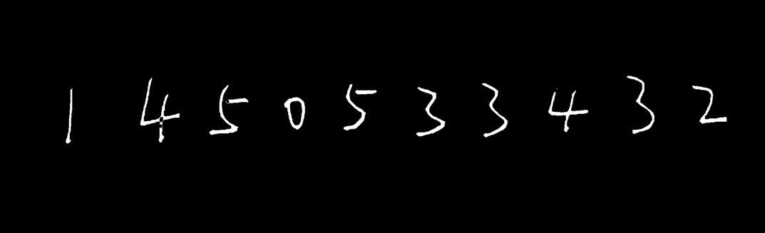
using Images #处理成能放入网络预测的28*28*1的矩阵

result = []

fillcolor = fill(RGB{Float32}(0), (1, 1))[1]

for i in 1:length(test_pic)

  if size(test_pic[i])[1] > 4 * size(test_pic[i])[2]

    z1 = zeros(Float32,size(test_pic[i])[1],2 * size(test_pic[i])[2])

    test_pic[i] = hcat(z1,hcat(test_pic[i],z1))

  end

  test_pic[i] = imresize(test_pic[i],(28,28),Pad=true,padcolor=fillcolor,stretch=false)

  input = reshape(test_pic[i]', 28,28,1,:) |>cpu

  load_result = model2(input) |>cpu #放入预测

  output = softmax(load_result) |>cpu

  push!(result,Flux.onecold(output, 0:9))

end
colorview(Gray,test_pic[4])

result
10-element Vector{Any}:

 [1]

 [4]

 [5]

 [0]

 [5]

 [3]

 [3]

 [4]

 [3]

 [2]
img
[cnn][julia]Flux实现卷积神经网络cnn预测手写MNIST的更多相关文章
- 【TensorFlow-windows】(四) CNN(卷积神经网络)进行手写数字识别(mnist)
主要内容: 1.基于CNN的mnist手写数字识别(详细代码注释) 2.该实现中的函数总结 平台: 1.windows 10 64位 2.Anaconda3-4.2.0-Windows-x86_64. ...
- 卷积神经网络CNN全面解析
卷积神经网络(CNN)概述 从多层感知器(MLP)说起 感知器 多层感知器 输入层-隐层 隐层-输出层 Back Propagation 存在的问题 从MLP到CNN CNN的前世今生 CNN的预测过 ...
- 【深度学习系列】手写数字识别卷积神经--卷积神经网络CNN原理详解(一)
上篇文章我们给出了用paddlepaddle来做手写数字识别的示例,并对网络结构进行到了调整,提高了识别的精度.有的同学表示不是很理解原理,为什么传统的机器学习算法,简单的神经网络(如多层感知机)都可 ...
- 深度学习之卷积神经网络(CNN)详解与代码实现(一)
卷积神经网络(CNN)详解与代码实现 本文系作者原创,转载请注明出处:https://www.cnblogs.com/further-further-further/p/10430073.html 目 ...
- 【深度学习系列】卷积神经网络CNN原理详解(一)——基本原理
上篇文章我们给出了用paddlepaddle来做手写数字识别的示例,并对网络结构进行到了调整,提高了识别的精度.有的同学表示不是很理解原理,为什么传统的机器学习算法,简单的神经网络(如多层感知机)都可 ...
- CNN学习笔记:卷积神经网络
CNN学习笔记:卷积神经网络 卷积神经网络 基本结构 卷积神经网络是一种层次模型,其输入是原始数据,如RGB图像.音频等.卷积神经网络通过卷积(convolution)操作.汇合(pooling)操作 ...
- 卷积神经网络CNN学习笔记
CNN的基本结构包括两层: 特征提取层:每个神经元的输入与前一层的局部接受域相连,并提取该局部的特征.一旦该局部特征被提取后,它与其它特征间的位置关系也随之确定下来: 特征映射层:网络的每个计算层由多 ...
- 深度学习之卷积神经网络CNN及tensorflow代码实现示例
深度学习之卷积神经网络CNN及tensorflow代码实现示例 2017年05月01日 13:28:21 cxmscb 阅读数 151413更多 分类专栏: 机器学习 深度学习 机器学习 版权声明 ...
- 卷积神经网络(CNN)前向传播算法
在卷积神经网络(CNN)模型结构中,我们对CNN的模型结构做了总结,这里我们就在CNN的模型基础上,看看CNN的前向传播算法是什么样子的.重点会和传统的DNN比较讨论. 1. 回顾CNN的结构 在上一 ...
- 卷积神经网络(CNN)反向传播算法
在卷积神经网络(CNN)前向传播算法中,我们对CNN的前向传播算法做了总结,基于CNN前向传播算法的基础,我们下面就对CNN的反向传播算法做一个总结.在阅读本文前,建议先研究DNN的反向传播算法:深度 ...
随机推荐
- Linux 身份验证被拒绝,登录失败解决
解决方案: vim /etc/ssh/sshd_config 修改参数 基本参数: PermitRootLogin yes #允许root认证登录 PasswordAuthentication yes ...
- 《深入理解Java虚拟机》读书笔记:Class类文件的结构
Class类文件的结构 Sun公司以及其他虚拟机提供商发布了许多可以运行在各种不同平台上的虚拟机,这些虚拟机都可以载入和执行同一种平台无关的的程序存储格式--字节码(ByteCode),从而实现了程序 ...
- 继copilot之后,又一款免费帮你写代码的插件
写在前面 在之前的文章中推荐过一款你写注释,它就能帮你写代码的插件copilot copilot写代码的能力没得说,但是呢copilot试用没几天之后就收费了 传送门:你写注释她帮你写代码 按理说这么 ...
- C#是否应该限制链式重载的设计模式?
1.代码的可阅读性 一眼看懂是什么意思,并且能看出生成的SQL是什么样的 var list = db.Queryable<Student>() .GroupBy(it => it.N ...
- 一次Python本地cache不当使用导致的内存泄露
背景 近期一个大版本上线后,Python编写的api主服务使用内存有较明显上升,服务重启后数小时就会触发机器的90%内存占用告警,分析后发现了本地cache不当使用导致的一个内存泄露问题,这里记录一下 ...
- DHorse v1.3.2 发布,基于 k8s 的发布平台
版本说明 新增特性 构建版本.部署应用时的线程池可配置化: 优化特性 构建版本跳过单元测试: 解决问题 解决Vue应用详情页面报错的问题: 解决Linux环境下脚本运行失败的问题: 解决下载Maven ...
- Nextcloud 维护管理
Nextcloud 维护管理 目录 Nextcloud 维护管理 1.管理员被禁用怎么办 2.管理员密码忘了怎么办 1.管理员被禁用怎么办 通过命令行解禁管理员用户: 方法一:通过命令行解禁管理员用户 ...
- Llama2-Chinese项目:1-项目介绍和模型推理
Atom-7B与Llama2间的关系:Atom-7B是基于Llama2进行中文预训练的开源大模型.为什么叫原子呢?因为原子生万物,Llama中文社区希望原子大模型未来可以成为构建AI世界的基础单位.目 ...
- 触动精灵生成的APK文件如何加固保护
触动精灵是一款模拟手机触摸.按键操作的软件,通过制作脚本,可以让触动精灵代替双手,自动执行一系列触摸.按键操作, 深受一些极客开发者喜爱. 触动精灵生成的APK文件自带了一些基础的加密,可以保护APK ...
- Kafka Stream 流和状态
4.2将状态操作应用到Kafka Stream 在上图的拓扑中生成了一个购买-交易事件流,拓扑中的一个处理节点根据销售额来计算客户的奖励级分.但在这个处理其中,要做的也仅仅时计算单笔交易的总积分,并转 ...