《DSP using MATLAB》示例Example6.29

代码：

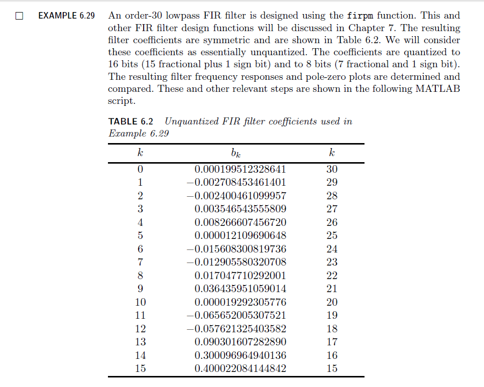
% The following funciton computes the filter
% coefficients shown in Table 6.2
b = firpm(30, [0, 0.3, 0.5, 1], [1, 1, 0, 0]);
w = [0:500]*pi/500; H = freqz(b, 1, w);
magH = abs(H); magHdb = 20*log10(magH);

% 16-bit word-length quantization
N1 = 15; [bhat1, L1, B1] = QCoeff(b, N1);
TITLE1 = sprintf('%i-bits (1+%i+%i) ', N1+1, L1, B1);
%bhat1 = bahat(1, :); ahat1 = bahat(2, :);
Hhat1 = freqz(bhat1, 1, w); magHhat1 = abs(Hhat1);
magHhat1db = 20*log10(magHhat1); zhat1 = roots(bhat1);

% 8-bit word-length quantization
N2 = 7; [bhat2, L2, B2] = QCoeff(b, N2);
TITLE2 = sprintf('%i-bits (1+%i+%i) ', N2+1, L2, B2);
%bhat2 = bahat(1, :); ahat2 = bahat(2, :);
Hhat2 = freqz(bhat2, 1, w); magHhat2 = abs(Hhat2);
magHhat2db = 20*log10(magHhat2); zhat2 = roots(bhat2);

% Comparison of Magnitude Plots
Hf_1 = figure('paperunits', 'inches', 'paperposition', [0, 0, 6, 5], 'NumberTitle', 'off', 'Name', 'Exameple 6.29');
%figure('NumberTitle', 'off', 'Name', 'Exameple 6.26a')
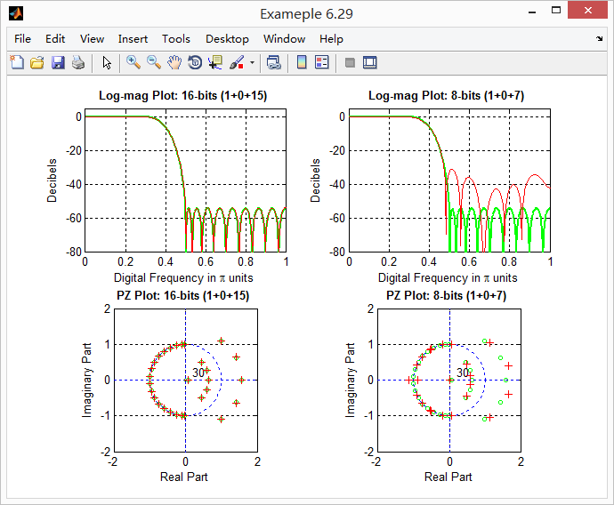
set(gcf,'Color','white');

% Comparison of Log-Magnitude Response: 16 bits
subplot(2, 2, 1); plot(w/pi, magHdb, 'g', 'linewidth', 1.5); axis([0, 1, -80, 5]);
hold on; plot(w/pi, magHhat1db, 'r', 'linewidth', 1); hold off;
xlabel('Digital Frequency in \pi units', 'fontsize', 10);
ylabel('Decibels', 'fontsize', 10); grid on;
title(['Log-mag Plot: ', TITLE1], 'fontsize', 10, 'fontweight', 'bold');

% Comparison of Pole-Zero Plots: 16 bits
subplot(2, 2, 3); [HZ, HP, Hl] = zplane([b], [1]); axis([-2, 2, -2, 2]); hold on;
set(HZ, 'color', 'g', 'linewidth', 1, 'markersize', 4);
set(HP, 'color', 'g', 'linewidth', 1, 'markersize', 4);
plot(real(zhat1), imag(zhat1), 'r+', 'linewidth', 1); grid on;
title(['PZ Plot: ' TITLE1], 'fontsize', 10, 'fontweight', 'bold'); hold off;

% Comparison of Log-Magnitude Response: 8 bits
subplot(2, 2, 2); plot(w/pi, magHdb, 'g', 'linewidth', 1.5); axis([0, 1, -80, 5]);
hold on; plot(w/pi, magHhat2db, 'r', 'linewidth', 1); hold off;
xlabel('Digital Frequency in \pi units', 'fontsize', 10);
ylabel('Decibels', 'fontsize', 10); grid on;
title(['Log-mag Plot: ', TITLE2], 'fontsize', 10, 'fontweight', 'bold');

% Comparison of Pole-Zero Plots: 8 bits
subplot(2, 2, 4); [HZ, HP, Hl] = zplane([b], [1]); axis([-2, 2, -2, 2]); hold on;
set(HZ, 'color', 'g', 'linewidth', 1, 'markersize', 4);
set(HP, 'color', 'g', 'linewidth', 1, 'markersize', 4);
plot(real(zhat2), imag(zhat2), 'r+', 'linewidth', 1); grid on;
title(['PZ Plot: ' TITLE2], 'fontsize', 10, 'fontweight', 'bold'); hold off;

运行结果：