plot a critical difference diagram , MATLAB code

建立criticaldifference函数

function cd = criticaldifference(s,labels,alpha)

%

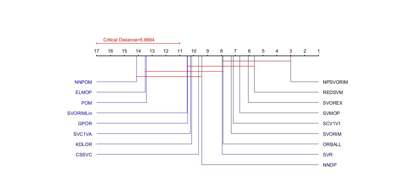
% CRITICALDIFFERNCE - plot a critical difference diagram

%

%    CRITICALDIFFERENCE(S,LABELS) produces a critical difference diagram [1]

%    displaying the statistical significance (or otherwise) of a matrix of

%    scores, S, achieved by a set of machine learning algorithms.  Here

%    LABELS is a cell array of strings giving the name of each algorithm.

%

%    References

%

%    [1] Demsar, J., "Statistical comparisons of classifiers over multiple

%        datasets", Journal of Machine Learning Research, vol. 7, pp. 1-30,

%        2006.

%

%

% File        : criticaldifference.m

%

% Date        : Monday 14th April 2008

%

% Author      : Gavin C. Cawley

%

% Description : Sparse multinomial logistic regression using a Laplace prior.

%

% History     : 14/04/2008 - v1.00

%

% Copyright   : (c) Dr Gavin C. Cawley, April 2008.

%

%    This program is free software; you can redistribute it and/or modify

%    it under the terms of the GNU General Public License as published by

%    the Free Software Foundation; either version 2 of the License, or

%    (at your option) any later version.

%

%    This program is distributed in the hope that it will be useful,

%    but WITHOUT ANY WARRANTY; without even the implied warranty of

%    MERCHANTABILITY or FITNESS FOR A PARTICULAR PURPOSE.  See the

%    GNU General Public License for more details.

%

%    You should have received a copy of the GNU General Public License

%    along with this program; if not, write to the Free Software

%    Foundation, Inc., 59 Temple Place, Suite 330, Boston, MA 02111-1307 USA

%

% Thanks to Gideon Dror for supplying the extended table of critical values.

if nargin < 3

   alpha = 0.1;

end

% convert scores into ranks

[N,k] = size(s);

[S,r] = sort(s');

idx   = k*repmat(0:N-1, k, 1)' + r';

R     = repmat(1:k, N, 1);

S     = S';

for i=1:N

    for j=1:k

        index    = S(i,j) == S(i,:);

        R(i,index) = mean(R(i,index));

    end

end

r(idx)  = R;

r       = r';

% compute critical difference

if alpha == 0.01

   qalpha = [0.000 2.576 2.913 3.113 3.255 3.364 3.452 3.526 3.590 3.646 ...

             3.696 3.741 3.781 3.818 3.853 3.884 3.914 3.941 3.967 3.992 ...

             4.015 4.037 4.057 4.077 4.096 4.114 4.132 4.148 4.164 4.179 ...

             4.194 4.208 4.222 4.236 4.249 4.261 4.273 4.285 4.296 4.307 ...

             4.318 4.329 4.339 4.349 4.359 4.368 4.378 4.387 4.395 4.404 ...

             4.412 4.420 4.428 4.435 4.442 4.449 4.456 ];

elseif alpha == 0.05

   qalpha = [0.000 1.960 2.344 2.569 2.728 2.850 2.948 3.031 3.102 3.164 ...

             3.219 3.268 3.313 3.354 3.391 3.426 3.458 3.489 3.517 3.544 ...

             3.569 3.593 3.616 3.637 3.658 3.678 3.696 3.714 3.732 3.749 ...

             3.765 3.780 3.795 3.810 3.824 3.837 3.850 3.863 3.876 3.888 ...

             3.899 3.911 3.922 3.933 3.943 3.954 3.964 3.973 3.983 3.992 ...

             4.001 4.009 4.017 4.025 4.032 4.040 4.046]; 

elseif alpha == 0.1

   qalpha = [0.000 1.645 2.052 2.291 2.460 2.589 2.693 2.780 2.855 2.920 ...

             2.978 3.030 3.077 3.120 3.159 3.196 3.230 3.261 3.291 3.319 ...

             3.346 3.371 3.394 3.417 3.439 3.459 3.479 3.498 3.516 3.533 ...

             3.550 3.567 3.582 3.597 3.612 3.626 3.640 3.653 3.666 3.679 ...

             3.691 3.703 3.714 3.726 3.737 3.747 3.758 3.768 3.778 3.788 ...

             3.797 3.806 3.814 3.823 3.831 3.838 3.846];

else

    error('alpha must be 0.01, 0.05 or 0.1');

end

cd = qalpha(k)*sqrt(k*(k+1)/(6*N));

figure(1);

clf

axis off

axis([-0.2 1.2 -20 140]);

axis xy

tics = repmat((0:(k-1))/(k-1), 3, 1);

line(tics(:), repmat([100, 101, 100], 1, k), 'LineWidth', 1.5, 'Color', 'k');

%tics = repmat(((0:(k-2))/(k-1)) + 0.5/(k-1), 3, 1);

%line(tics(:), repmat([100, 101, 100], 1, k-1), 'LineWidth', 1.5, 'Color', 'k');

line([0 0 0 cd/(k-1) cd/(k-1) cd/(k-1)], [113 111 112 112 111 113], 'LineWidth', 1, 'Color', 'r');

text(0.03, 116, ['Critical Distance=' num2str(cd)], 'FontSize', 12, 'HorizontalAlignment', 'left', 'Color', 'r');

for i=1:k

    text((i-1)/(k-1), 105, num2str(k-i+1), 'FontSize', 12, 'HorizontalAlignment', 'center');

end

% compute average ranks

r       = mean(r);

[r,idx] = sort(r);

% compute statistically similar cliques

clique           = repmat(r,k,1) - repmat(r',1,k);

clique(clique<0) = realmax;

clique           = clique < cd;

for i=k:-1:2

    if all(clique(i-1,clique(i,:))==clique(i,clique(i,:)))

        clique(i,:) = 0;

    end

end

n                = sum(clique,2);

clique           = clique(n>1,:);

n                = size(clique,1);

%yanse={'b','g','y','m','r'};

b=linspace(0,1,k);

% labels displayed on the right

for i=1:ceil(k/2)

   line([(k-r(i))/(k-1) (k-r(i))/(k-1) 1], [100 100-3*(n+1)-10*i 100-3*(n+1)-10*i], 'Color', [0 0 b(i)]);

   %text(1.2, 100 - 5*(n+1)- 10*i + 2, num2str(r(i)), 'FontSize', 10, 'HorizontalAlignment', 'right');

   text(1.02, 100 - 3*(n+1) - 10*i, labels{idx(i)}, 'FontSize', 12, 'VerticalAlignment', 'middle', 'HorizontalAlignment', 'left', 'Color', [0 0 b(i)]);

end

% labels displayed on the left

for i=ceil(k/2)+1:k

   line([(k-r(i))/(k-1) (k-r(i))/(k-1) 0], [100 100-3*(n+1)-10*(k-i+1) 100-3*(n+1)-10*(k-i+1)], 'Color', [0 0 b(i)]);

   %text(-0.2, 100 - 5*(n+1) -10*(k-i+1)+2, num2str(r(i)), 'FontSize', 10, 'HorizontalAlignment', 'left');

   text(-0.02, 100 - 3*(n+1) -10*(k-i+1), labels{idx(i)}, 'FontSize', 12, 'VerticalAlignment', 'middle', 'HorizontalAlignment', 'right', 'Color', [0 0 b(i)]);

end

% group cliques of statistically similar classifiers

for i=1:size(clique,1)

   R = r(clique(i,:));

   %line([((k-min(R))/(k-1)) + 0.015 ((k - max(R))/(k-1)) - 0.015], [100-5*i 100-5*i], 'LineWidth', 1, 'Color', 'r');

   %line([0 0 0 cd/(k-1) cd/(k-1) cd/(k-1)], [113 111 112 112 111 113], 'LineWidth', 1, 'Color', 'r');

   line([((k-min(R))/(k-1)) ((k-min(R))/(k-1)) ((k-min(R))/(k-1)) ((k - max(R))/(k-1)) ((k - max(R))/(k-1)) ((k - max(R))/(k-1))], [100+1-5*i 100-1-5*i 100-5*i 100-5*i 100-1-5*i 100+1-5*i], 'LineWidth', 1, 'Color', 'r');

end

　可执行m文件：

 load Data

s=AccMatrix;

labels={'SCV1V1','SVC1VA','SVR','CSSVC','SVMOP','NNOP','ELMOP','POM',...

    'NNPOM', 'SVOREX','SVORIM','SVORIMLin','KDLOR','GPOR','REDSVM','ORBALL' ,'NPSVORIM'};%方法的标签

alpha=0.05; %显著性水平0.1,0.05或0.01

cd = criticaldifference(s,labels,alpha)

　　AccMatrix=[

0.28 0.12 0.28 0.11 0.32 0.08 0.26 0.13 0.37 0.10 0.28 0.12 0.42 0.21 0.38 0.17 0.36 0.14 0.36 0.13 0.38 0.12 0.37 0.10 0.34 0.15 0.39 0.09 0.37 0.12 0.36 0.13 0.37 0.11

0.31 0.12 0.33 0.11 0.34 0.13 0.32 0.11 0.32 0.09 0.24 0.11 0.40 0.18 0.50 0.15 0.34 0.18 0.35 0.12 0.34 0.12 0.34 0.12 0.33 0.11 0.48 0.17 0.33 0.11 0.30 0.12 0.28 0.14

0.36 0.09 0.40 0.14 0.39 0.11 0.39 0.13 0.40 0.09 0.39 0.11 0.44 0.16 0.62 0.15 0.50 0.13 0.37 0.13 0.37 0.13 0.37 0.13 0.39 0.12 0.55 0.10 0.38 0.13 0.36 0.12 0.32 0.10

0.22 0.12 0.28 0.16 0.24 0.10 0.27 0.15 0.27 0.11 0.29 0.11 0.39 0.13 0.65 0.14 0.39 0.14 0.26 0.11 0.27 0.11 0.32 0.11 0.26 0.11 0.36 0.16 0.27 0.12 0.30 0.10 0.22 0.10

0.44 0.06 0.45 0.06 0.40 0.07 0.43 0.07 0.46 0.06 0.41 0.06 0.44 0.08 0.50 0.08 0.45 0.09 0.41 0.07 0.40 0.07 0.48 0.07 0.43 0.05 0.67 0.04 0.40 0.07 0.40 0.06 0.41 0.05

0.03 0.03 0.04 0.03 0.04 0.02 0.04 0.02 0.04 0.03 0.04 0.02 0.06 0.02 0.03 0.02 0.03 0.03 0.03 0.02 0.03 0.02 0.03 0.02 0.03 0.02 0.03 0.02 0.03 0.02 0.04 0.03 0.03 0.03

0.03 0.01 0.03 0.01 0.16 0.03 0.03 0.01 0.03 0.01 0.04 0.01 0.09 0.02 0.09 0.02 0.06 0.05 0.00 0.01 0.00 0.01 0.09 0.02 0.16 0.03 0.03 0.01 0.00 0.00 0.03 0.02 0.02 0.01

0.42 0.03 0.44 0.03 0.43 0.03 0.43 0.03 0.42 0.03 0.42 0.03 0.43 0.02 0.43 0.03 0.46 0.03 0.43 0.03 0.43 0.03 0.43 0.03 0.51 0.03 0.42 0.03 0.43 0.03 0.44 0.03 0.43 0.03

0.01 0.00 0.01 0.01 0.03 0.01 0.01 0.01 0.00 0.00 0.03 0.01 0.16 0.01 0.84 0.30 0.11 0.02 0.01 0.01 0.01 0.01 0.08 0.01 0.05 0.01 0.04 0.01 0.01 0.00 0.01 0.01 0.01 0.00

0.43 0.04 0.43 0.06 0.46 0.07 0.43 0.06 0.45 0.10 0.53 0.09 0.57 0.13 0.66 0.16 0.62 0.14 0.45 0.06 0.45 0.07 0.43 0.08 0.47 0.09 0.42 0.03 0.44 0.05 0.46 0.09 0.42 0.08

0.05 0.03 0.05 0.03 0.07 0.04 0.05 0.03 0.07 0.03 0.06 0.03 0.07 0.03 0.71 0.03 0.06 0.03 0.02 0.01 0.02 0.01 0.74 0.01 0.11 0.03 0.05 0.02 0.02 0.01 0.05 0.02 0.04 0.03

0.36 0.03 0.45 0.03 0.36 0.03 0.44 0.03 0.35 0.03 0.42 0.04 0.43 0.03 0.85 0.02 0.46 0.04 0.36 0.03 0.36 0.03 0.36 0.02 0.37 0.03 0.31 0.03 0.36 0.03 0.38 0.03 0.34 0.03

0.37 0.02 0.37 0.02 0.38 0.02 0.37 0.02 0.37 0.02 0.37 0.03 0.37 0.02 0.38 0.03 0.38 0.02 0.38 0.02 0.38 0.02 0.39 0.02 0.46 0.03 0.39 0.03 0.37 0.02 0.39 0.03 0.37 0.03

0.25 0.06 0.26 0.06 0.32 0.07 0.27 0.06 0.26 0.04 0.39 0.06 0.38 0.06 0.53 0.19 0.55 0.08 0.32 0.05 0.32 0.07 0.41 0.07 0.30 0.07 0.39 0.07 0.32 0.07 0.29 0.05 0.27 0.05

0.35 0.02 0.36 0.02 0.37 0.02 0.36 0.02 0.36 0.02 0.40 0.02 0.40 0.02 0.40 0.02 0.40 0.02 0.37 0.02 0.37 0.02 0.41 0.02 0.35 0.02 0.39 0.01 0.37 0.02 0.33 0.02 0.36 0.02

0.31 0.04 0.33 0.03 0.30 0.03 0.32 0.03 0.29 0.03 0.31 0.04 0.30 0.04 0.29 0.03 0.34 0.13 0.29 0.03 0.28 0.03 0.29 0.04 0.36 0.03 0.29 0.03 0.29 0.03 0.32 0.02 0.29 0.03

0.74 0.02 0.82 0.03 0.75 0.02 0.80 0.03 0.74 0.02 0.71 0.02 0.75 0.02 0.74 0.02 0.73 0.03 0.71 0.03 0.75 0.02 0.76 0.02 0.81 0.03 0.71 0.03 0.75 0.02 0.76 0.02 0.75 0.03 ];

plot a critical difference diagram , MATLAB code的更多相关文章

Silence Removal and End Point Detection MATLAB Code
转载自:http://ganeshtiwaridotcomdotnp.blogspot.com/2011/08/silence-removal-and-end-point-detection.html ...
Compute Mean Value of Train and Test Dataset of Caltech-256 dataset in matlab code
Compute Mean Value of Train and Test Dataset of Caltech-256 dataset in matlab code clc;imPath = '/ho ...
Matlab Code for Visualize the Tracking Results of OTB100 dataset
Matlab Code for Visualize the Tracking Results of OTB100 dataset 2018-11-12 17:06:21 %把所有tracker的结果画 ...
支持向量机的smo算法（MATLAB code）
建立smo.m % function [alpha,bias] = smo(X, y, C, tol) function model = smo(X, y, C, tol) % SMO: SMO al ...
MFCC matlab code
%function ccc=mfcc(x) %归一化mel滤波器组系数 filename=input('input filename:','s'); [x,fs,bits]=wavread(filen ...
word linkage 选择合适的聚类个数matlab code
clear load fisheriris X = meas; m = size(X,2); % load machine % load census % % X = meas; % X=X(1:20 ...
sequential minimal optimization,SMO for SVM, (MATLAB code)
function model = SMOforSVM(X, y, C ) %sequential minimal optimization,SMO tol = 0.001; maxIters = 30 ...
MATLAB中矢量场图的绘制 (quiver/quiver3/dfield/pplane) Plot the vector field with MATLAB
1.quiver函数一般用于绘制二维矢量场图,函数调用方法如下: quiver(x,y,u,v) 该函数展示了点(x,y)对应的的矢量(u,v).其中,x的长度要求等于u.v的列数,y的长度要求等于 ...
求平均排序MATLAB code
A0=R(:,1:2:end); for i=1:17 A1=A0(i,:); p=sort(unique(A1)); for j=1:length(p) Rank0(A1==p(j))=j; end ...

随机推荐

Beaglebone Black - 准备
首先要玩 BBB,你需要买一台 BBB,淘宝 Element14 Beaglebone Black,我购入价 RMB 310,带数据线,没电源适配器的.Seeedstudio 有台叫 Beaglebo ...
JDBC操作Oracle数据库
背景知识含义:JDBC是一种java数据库连接技术,能实现java程序对各种数据库的访问.由一组使用java语言编写的类和接口组成,这些类和接口称为JDBC API,他们位于java.sql 以及j ...
PostgresSql开放局域网访问
1) 确认已经退掉所有的MASF终端和MSF GUI,然后打开PostgresSQL的启动文件在文件POSTGRESQL_START参数后面添加-h 0.0.0.0,让PostgreSQL启动时绑定到 ...
NSValue
1.利用NSValue包装自定义的结构体 typedef struct{ int age; char *name; double height; ...
Perfection Kills
<!doctype html> <html> <head> <meta charset="utf-8"> <title> ...
Mybatis Generator（定制化）代码生成器
1.使用Mapper专用的MyBatis Generator插件通用Mapper在1.0.0版本的时候增加了MyBatis Generator(以下简称MBG)插件,使用该插件可以很方便的生成实体类 ...
Redis基础知识之————如何处理客户端连接
redis 连接建立 Redis Redis 通过监听一个 TCP 端口或者 Unix socket 的方式来接收来自客户端的连接,当一个连接建立后,Redis 内部会进行以下一些操作: 首先,客户端 ...
JavaWeb学习总结（十一）--JDBC之批处理
一.批处理的介绍在实际的项目开发中,有时候需要向数据库发送一批SQL语句执行,这时应避免向数据库一条条的发送执行,而应采用JDBC的批处理机制,以提升执行效率.批处理只针对更新(增.删.改)语句,批 ...
Binary Tree Paths
Description: Given a binary tree, return all root-to-leaf paths. For example, given the following bi ...
JS重要知识点(转载学习中。。。)
这里列出了一些JS重要知识点(不全面,但自己感觉很重要).彻底理解并掌握这些知识点,对于每个想要深入学习JS的朋友应该都是必须的. 讲解还是以示例代码搭配注释的形式,这里做个小目录: JS代码预解析原 ...

plot a critical difference diagram , MATLAB code

plot a critical difference diagram , MATLAB code的更多相关文章

随机推荐

热门专题