角点检测和匹配——Harris算子

一、基本概念

角点corner：可以将角点看做两个边缘的交叉处，在两个方向上都有较大的变化。具体可由下图中分辨出来：

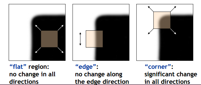
兴趣点interest point：兴趣点是图像中能够较鲁棒的检测出来的点，它不仅仅局限于角点. 也可以是灰度图像极大值或者极小值点等

二、Harris角点检测

Harris 算子是 Haris & Stephens 1988年在 "A Combined Corner and Edge Detector" 中提出的 提出的检测算法, 现在已经成为图像匹配中常用的算法.

对于一幅RGB图像我们很很容易得到corner 是各个方向梯度值较大的点, 定义 函数WSSD(Weighted Sum Squared Difference)为：

$$S(x,y) = \sum_{u} \sum_{v}w(u,v)(I((u+x,v+y)-I(u,v))^2 (1)$$

其中$w(u,v)$可以看作采样窗，可以选择矩形窗函数，也可以选择高斯窗函数:

$I(u+x,v+y)-I(u,v)$可以看作像素值变化量(梯度):

使用泰勒展开:$I(u+x,v+y) \approx I(u,v)+I_x(u,v)x+I_y(u,v)y (2)$

(1)代入(2) $S(x,y) \approx \sum_u \sum_v w(u,v) (I_x(u,v)x + I_y(u,v)y)^2$

写成$S(x,y) \approx (x,y) A (x,y)^T $

其中 A 为 二阶梯度矩阵(structure tensor/ second-moment matrix)

$$A = \sum_u \sum_v w(u,v) \begin{bmatrix} I_x^2& I_x I_y \\ I_x I_y & I_y^2 \end{bmatrix} $$

将A定义为Harris Matrix,A 的特征值有三种情况：

1. $\lambda_1 \approx 0, \lambda_2 \approx 0$，那么点$x$不是兴趣点

2. $\lambda_1 \approx 0, \lambda_2$为一个较大的正数, 那么点$x$为边缘点(edge)

3. $\lambda_1, \lambda_2$都为一个较大的正数, 那么点$x$为角点(corner)

由于特征值的计算是 computationally expensive，引入如下函数

$M_c = \lambda_1\lambda_2 - \kappa(\lambda_1+\lambda_2)^2 = det(A) - \kappa trace^2(A) $

为了去除加权常数$\kappa$ 直接计算

$M_{c}^{'}  =  \frac{det(A)}{trace(A)+\epsilon}$

三、角点匹配

Harris角点检测仅仅检测出兴趣点位置，然而往往我们进行角点检测的目的是为了进行图像间的兴趣点匹配，我们在每一个兴趣点加入descriptors描述子信息，给出比较描述子信息的方法. Harris角点的，描述子是由周围像素值块batch的灰度值，以及用于比较归一化的相关矩阵构成。

通常，两个大小相同的像素块I_1(x)和I_2(x) 的相关矩阵为:
$$c(I_1,I_2) = \sum_x f(I_1(x),I_2(x))$$

$f函数随着方法变化而变化,c(I_1,I_2)$值越大，像素块相似度越高.

对互相关矩阵进行归一化得到normalized cross correlation :

$$ncc(I_1,I_2) = \frac{1}{n-2} \sum_x \frac{(I_1(x)-\mu_1)}{\sigma_1} \cdot \frac{(I_2(x)-\mu_2)}{\sigma_2}$$

其中$\mu$为像素块的均值，\sigma为标准差. ncc对图像的亮度变化具有更好的稳健性.

四、python实现

python版本:2.7

依赖包: numpy,scipy,PIL, matplotlib

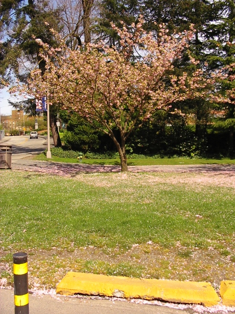
图片：

trees_002.jpg

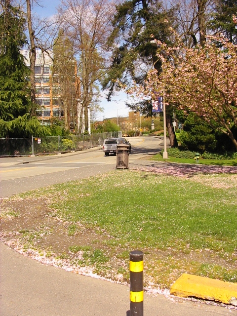
trees003.jpg

from PIL import Image
from scipy.ndimage import filters
from numpy import *
from pylab import *

def compute_harris_response(im,sigma=3):
    """Compute the Harris corner detector response function for each
    pixel in a graylevel image."""

    #derivative
    imx = zeros(im.shape)
    filters.gaussian_filter(im,(sigma,sigma),(0,1),imx)

    imy = zeros(im.shape)
    filters.gaussian_filter(im,(sigma,sigma),(1,0),imy)

    #compute components of the Harris matrix

    Wxx = filters.gaussian_filter(imx*imx,sigma)
    Wxy = filters.gaussian_filter(imx*imy,sigma)
    Wyy = filters.gaussian_filter(imy*imy,sigma)

    #determinant and trace

    Wdet = Wxx*Wyy-Wxy**2
    Wtr = Wxx+Wyy
    return Wdet/Wtr

def get_harris_points(harrisim,min_dist=10,threshold=0.1):
    """Return corners from a Harris response image min_dist is the
    minimum number of pixels separating corners and image boundary."""

    #find top corner candidates above a threshold
    corner_threshold  = harrisim.max()*threshold
    harrisim_t = 1*(harrisim>corner_threshold)

    #get coordiantes of candidate
    coords = array(harrisim_t.nonzero()).T

    #...and their valus
    candicates_values = [harrisim[c[0],c[1]] for c in coords]

    #sort candicates
    index = argsort(candicates_values)

    #sort allowed point loaction in array
    allowed_location = zeros(harrisim.shape)
    allowed_location[min_dist:-min_dist,min_dist:-min_dist] = 1

    #select the best points taking min_distance into account
    filtered_coords = []
    for i in index:
        if  allowed_location[coords[i,0],coords[i,1]]==1:
            filtered_coords.append(coords[i])
            allowed_location[(coords[i,0]-min_dist):(coords[i,0]+min_dist),
                              (coords[i,1]-min_dist):(coords[i,1]+min_dist)]=0
    return filtered_coords

def plot_harris_points(image,filtered_coords):
    """plots corners found in image."""
    figure
    gray()
    imshow(image)
    plot([p[1] for p in filtered_coords],[p[0] for p in filtered_coords],'*')
    axis('off')
    show()

def get_descriptors(image,filter_coords,wid=5):
    """For each point return pixel values around the point using a neihborhood
    of 2*width+1."""
    desc=[]
    for coords in filter_coords:
        patch = image[coords[0]-wid:coords[0]+wid+1,
                      coords[1]-wid:coords[1]+wid+1].flatten()
        desc.append(patch) # use append to add new elements
    return desc

def match(desc1,desc2,threshold=0.5):
    """For each corner point descriptor in the first image, select its match
    to second image using normalized cross correlation."""

    n = len(desc1[0]) #num of harris descriptors
    #pair-wise distance
    d = -ones((len(desc1),len(desc2)))
    for i in range(len(desc1)):
        for j in range(len(desc2)):
            d1 = (desc1[i]-mean(desc1[i]))/std(desc1[i])
            d2 = (desc2[j]-mean(desc2[j]))/std(desc2[j])
            ncc_value = sum(d1*d2)/(n-1)
            if ncc_value>threshold:
                d[i,j] = ncc_value

    ndx = argsort(-d)
    matchscores = ndx[:,0]

    return matchscores

def match_twosided(desc1,desc2,threshold=0.5):
    """two sided symmetric version of match()."""
    matches_12 = match(desc1,desc2,threshold)
    matches_21 = match(desc2,desc1,threshold)

    ndx_12 = where(matches_12>=0)[0]
    print ndx_12.dtype
    # remove matches that are not symmetric
    for n in ndx_12:
        if matches_21[matches_12[n]] !=n:
            matches_12[n] = -1
    return matches_12    

def appendimages(im1,im2):
    """Return a new image that appends that two images side-by-side."""

    #select the image with the fewest rows and fill in enough empty rows
    rows1 = im1.shape[0]
    rows2 = im2.shape[0]

    if rows1<rows2:
        im1 = concatenate((im1,zeros((rows2-rows1,im1.shape[1]))),axis=0)
    elif rows1<rows2:
        im2 = concatenate((im2,zeros((rows1-rows2,im2.shape[1]))),axis=0)
    return concatenate((im1,im2),axis=1)
def plot_matches(im1,im2,locs1,locs2,matchscores,show_below=True):
    """show a figure with lines joinging the accepted matches
    Input:im1,im2(images as arrays),locs1,locs2,(feature locations),
          metachscores(as output from 'match()'),
          show_below(if images should be shown matches)."""
    im3 = appendimages(im1,im2)
    if show_below:
        im3 = vstack((im3,im3))

    imshow(im3)

    cols1 = im1.shape[1]
    for i,m in enumerate(matchscores):
        if m>0:
            plot([locs1[i][1],locs2[m][1]+cols1],[locs1[i][0],locs2[m][0]],'c')
    axis('off')

"""
im = array(Image.open('F:/images/lena.bmp').convert('1'))
harrisim = compute_harris_response(im)
filtered_coords = get_harris_points(harrisim,6)
plot_harris_points(im,filtered_coords)
"""

im1 = array(Image.open('trees_002.jpg').convert('L'))
im2 = array(Image.open('trees_003.jpg').convert('L'))

wid = 5

harrisim = compute_harris_response(im1,5)
filtered_coords1 = get_harris_points(harrisim,wid+1)
d1 = get_descriptors(im1,filtered_coords1,wid)

harrisim = compute_harris_response(im2,5)
filtered_coords2 = get_harris_points(harrisim,wid+1)
d2 = get_descriptors(im2,filtered_coords2,wid)

print 'starting matching'
matches = match_twosided(d1,d2)

figure()
gray()
plot_matches(im1,im2,filtered_coords1,filtered_coords2,matches)
show()

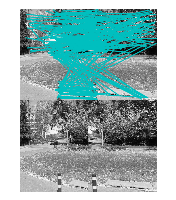
运行结果: