深度学习基础系列(十)| Global Average Pooling是否可以替代全连接层?
Global Average Pooling(简称GAP,全局池化层)技术最早提出是在这篇论文(第3.2节)中,被认为是可以替代全连接层的一种新技术。在keras发布的经典模型中,可以看到不少模型甚至抛弃了全连接层,转而使用GAP,而在支持迁移学习方面,各个模型几乎都支持使用Global Average Pooling和Global Max Pooling(GMP)。 然而,GAP是否真的可以取代全连接层?其背后的原理何在呢?本文来一探究竟。
一、什么是GAP?
先看看原论文的定义:
In this paper, we propose another strategy called global average pooling to replace the traditional fully connected layers in CNN. The idea is to generate one feature map for each corresponding category of the classification task in the last mlpconv layer. Instead of adding fully connected layers on top of the feature maps, we take the average of each feature map, and the resulting vector is fed directly into the softmax layer. One advantage of global average pooling over the fully connected layers is that it is more native to the convolution structure by enforcing correspondences between feature maps and categories. Thus the feature maps can be easily interpreted as categories confidence maps. Another advantage is that there is no parameter to optimize in the global average pooling thus overfitting is avoided at this layer. Futhermore, global average pooling sums out the spatial information, thus it is more robust to spatial translations of the input.
简单来说,就是在卷积层之后,用GAP替代FC全连接层。有两个有点:一是GAP在特征图与最终的分类间转换更加简单自然;二是不像FC层需要大量训练调优的参数,降低了空间参数会使模型更加健壮,抗过拟合效果更佳。
我们再用更直观的图像来看GAP的工作原理:
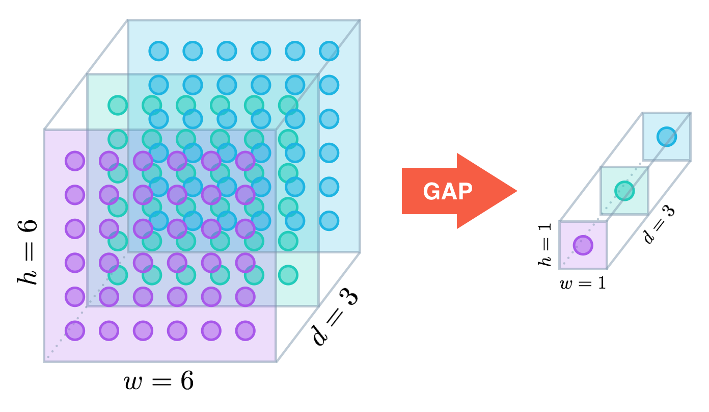
假设卷积层的最后输出是h × w × d 的三维特征图,具体大小为6 × 6 × 3,经过GAP转换后,变成了大小为 1 × 1 × 3 的输出值,也就是每一层 h × w 会被平均化成一个值。
二、 GAP在Keras中的定义
GAP的使用一般在卷积层之后,输出层之前:
x = layers.MaxPooling2D((2, 2), strides=(2, 2), name='block5_pool')(x) #卷积层最后一层

x = layers.GlobalAveragePooling2D()(x) #GAP层

prediction = Dense(10, activation='softmax')(x) #输出层
再看看GAP的代码具体实现:
@tf_export('keras.layers.GlobalAveragePooling2D',

           'keras.layers.GlobalAvgPool2D')

class GlobalAveragePooling2D(GlobalPooling2D):

  """Global average pooling operation for spatial data.

  Arguments:

      data_format: A string,

          one of `channels_last` (default) or `channels_first`.

          The ordering of the dimensions in the inputs.

          `channels_last` corresponds to inputs with shape

          `(batch, height, width, channels)` while `channels_first`

          corresponds to inputs with shape

          `(batch, channels, height, width)`.

          It defaults to the `image_data_format` value found in your

          Keras config file at `~/.keras/keras.json`.

          If you never set it, then it will be "channels_last".

  Input shape:

      - If `data_format='channels_last'`:

          4D tensor with shape:

          `(batch_size, rows, cols, channels)`

      - If `data_format='channels_first'`:

          4D tensor with shape:

          `(batch_size, channels, rows, cols)`

  Output shape:

      2D tensor with shape:

      `(batch_size, channels)`

  """

  def call(self, inputs):

    if self.data_format == 'channels_last':

      return backend.mean(inputs, axis=[1, 2])

    else:

      return backend.mean(inputs, axis=[2, 3])
实现很简单,对宽度和高度两个维度的特征数据进行平均化求值。如果是NHWC结构(数量、宽度、高度、通道数),则axis=[1, 2];反之如果是CNHW,则axis=[2, 3]。
三、GAP VS GMP VS FC
在验证GAP技术可行性前,我们需要准备训练和测试数据集。我在牛津大学网站上找到了17种不同花类的数据集,地址为:http://www.robots.ox.ac.uk/~vgg/data/flowers/17/index.html 。该数据集每种花有80张图片,共计1360张图片,我对花进行了分类处理,抽取了部分数据作为测试数据,这样最终训练和测试数据的数量比为7:1。
我将数据集上传到我的百度网盘: https://pan.baidu.com/s/1YDA_VOBlJSQEijcCoGC60w ,大家可以下载使用。
在Keras经典模型中,若支持迁移学习,不但有GAP,还有GMP,而默认是自己组建FC层,一个典型的实现为:
 if include_top:

        # Classification block

        x = layers.Flatten(name='flatten')(x)

        x = layers.Dense(4096, activation='relu', name='fc1')(x)

        x = layers.Dense(4096, activation='relu', name='fc2')(x)

        x = layers.Dense(classes, activation='softmax', name='predictions')(x)

    else:

        if pooling == 'avg':

            x = layers.GlobalAveragePooling2D()(x)

        elif pooling == 'max':

            x = layers.GlobalMaxPooling2D()(x)
本文将在同一数据集条件下,比较GAP、GMP和FC层的优劣,选取测试模型为VGG19和InceptionV3两种模型的迁移学习版本。
先看看在VGG19模型下,GAP、GMP和FC层在各自迭代50次后,验证准确度和损失度的比对。代码如下:
import keras

from keras.preprocessing.image import ImageDataGenerator

from keras.models import Model

from keras.applications.vgg19 import VGG19from keras.layers import Dense, Flatten

from matplotlib import pyplot as plt

import numpy as np

# 为保证公平起见,使用相同的随机种子

np.random.seed(7)

batch_size = 32

# 迭代50次

epochs = 50

# 依照模型规定,图片大小被设定为224

IMAGE_SIZE = 224

# 17种花的分类

NUM_CLASSES = 17

TRAIN_PATH = '/home/yourname/Documents/tensorflow/images/17flowerclasses/train'

TEST_PATH = '/home/yourname/Documents/tensorflow/images/17flowerclasses/test'

FLOWER_CLASSES = ['Bluebell', 'ButterCup', 'ColtsFoot', 'Cowslip', 'Crocus', 'Daffodil', 'Daisy',

                  'Dandelion', 'Fritillary', 'Iris', 'LilyValley', 'Pansy', 'Snowdrop', 'Sunflower',

                  'Tigerlily', 'tulip', 'WindFlower']

def model(mode='fc'):

    if mode == 'fc':

        # FC层设定为含有512个参数的隐藏层

        base_model = VGG19(input_shape=(IMAGE_SIZE, IMAGE_SIZE, 3), include_top=False, pooling='none')

        x = base_model.output

        x = Flatten()(x)

        x = Dense(512, activation='relu')(x)

        prediction = Dense(NUM_CLASSES, activation='softmax')(x)

    elif mode == 'avg':

        # GAP层通过指定pooling='avg'来设定

        base_model = VGG19(input_shape=(IMAGE_SIZE, IMAGE_SIZE, 3), include_top=False, pooling='avg')

        x = base_model.output

        prediction = Dense(NUM_CLASSES, activation='softmax')(x)

    else:

        # GMP层通过指定pooling='max'来设定

        base_model = VGG19(input_shape=(IMAGE_SIZE, IMAGE_SIZE, 3), include_top=False, pooling='max')

        x = base_model.output

        prediction = Dense(NUM_CLASSES, activation='softmax')(x)

    model = Model(input=base_model.input, output=prediction)

    model.summary()

    opt = keras.optimizers.rmsprop(lr=0.0001, decay=1e-6)

    model.compile(loss='categorical_crossentropy',

                             optimizer=opt,

                             metrics=['accuracy'])

    # 使用数据增强

    train_datagen = ImageDataGenerator()

    train_generator = train_datagen.flow_from_directory(directory=TRAIN_PATH,

                                                        target_size=(IMAGE_SIZE, IMAGE_SIZE),

                                                        classes=FLOWER_CLASSES)

    test_datagen = ImageDataGenerator()

    test_generator = test_datagen.flow_from_directory(directory=TEST_PATH,

                                                      target_size=(IMAGE_SIZE, IMAGE_SIZE),

                                                      classes=FLOWER_CLASSES)

    # 运行模型

    history = model.fit_generator(train_generator, epochs=epochs, validation_data=test_generator)

    return history

fc_history = model('fc')

avg_history = model('avg')

max_history = model('max')

# 比较多种模型的精确度

plt.plot(fc_history.history['val_acc'])

plt.plot(avg_history.history['val_acc'])

plt.plot(max_history.history['val_acc'])

plt.title('Model accuracy')

plt.ylabel('Validation Accuracy')

plt.xlabel('Epoch')

plt.legend(['FC', 'AVG', 'MAX'], loc='lower right')

plt.grid(True)

plt.show()

# 比较多种模型的损失率

plt.plot(fc_history.history['val_loss'])

plt.plot(avg_history.history['val_loss'])

plt.plot(max_history.history['val_loss'])

plt.title('Model loss')

plt.ylabel('Loss')

plt.xlabel('Epoch')

plt.legend(['FC', 'AVG', 'MAX'], loc='upper right')

plt.grid(True)

plt.show()
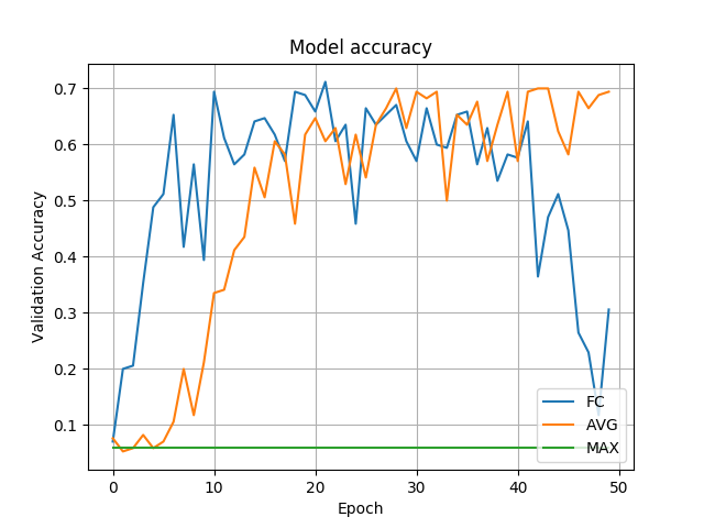
各自运行50次迭代后,我们看看准确度比较:
再看看损失度比较:
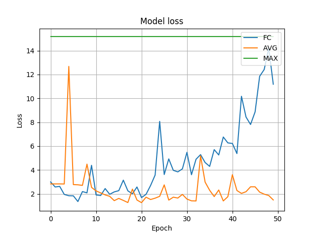
可以看出,首先GMP在本模型中表现太差,不值一提;而FC在前40次迭代时表现尚可,但到了40次后发生了剧烈变化,出现了过拟合现象(运行20次左右时的模型相对较好,但准确率不足70%,模型还是很差);三者中表现最好的是GAP,无论从准确度还是损失率,表现都较为平稳,抗过拟合化效果明显(但最终的准确度70%,模型还是不行)。
我们再转向另一个模型InceptionV3,代码稍加改动如下:
import keras

from keras.preprocessing.image import ImageDataGenerator

from keras.models import Model

from keras.applications.inception_v3 import InceptionV3, preprocess_input

from keras.layers import Dense, Flatten

from matplotlib import pyplot as plt

import numpy as np

# 为保证公平起见,使用相同的随机种子

np.random.seed(7)

batch_size = 32

# 迭代50次

epochs = 50

# 依照模型规定,图片大小被设定为224

IMAGE_SIZE = 224

# 17种花的分类

NUM_CLASSES = 17

TRAIN_PATH = '/home/hutao/Documents/tensorflow/images/17flowerclasses/train'

TEST_PATH = '/home/hutao/Documents/tensorflow/images/17flowerclasses/test'

FLOWER_CLASSES = ['Bluebell', 'ButterCup', 'ColtsFoot', 'Cowslip', 'Crocus', 'Daffodil', 'Daisy',

                  'Dandelion', 'Fritillary', 'Iris', 'LilyValley', 'Pansy', 'Snowdrop', 'Sunflower',

                  'Tigerlily', 'tulip', 'WindFlower']

def model(mode='fc'):

    if mode == 'fc':

        # FC层设定为含有512个参数的隐藏层

        base_model = InceptionV3(input_shape=(IMAGE_SIZE, IMAGE_SIZE, 3), include_top=False, pooling='none')

        x = base_model.output

        x = Flatten()(x)

        x = Dense(512, activation='relu')(x)

        prediction = Dense(NUM_CLASSES, activation='softmax')(x)

    elif mode == 'avg':

        # GAP层通过指定pooling='avg'来设定

        base_model = InceptionV3(input_shape=(IMAGE_SIZE, IMAGE_SIZE, 3), include_top=False, pooling='avg')

        x = base_model.output

        prediction = Dense(NUM_CLASSES, activation='softmax')(x)

    else:

        # GMP层通过指定pooling='max'来设定

        base_model = InceptionV3(input_shape=(IMAGE_SIZE, IMAGE_SIZE, 3), include_top=False, pooling='max')

        x = base_model.output

        prediction = Dense(NUM_CLASSES, activation='softmax')(x)

    model = Model(input=base_model.input, output=prediction)

    model.summary()

    opt = keras.optimizers.rmsprop(lr=0.0001, decay=1e-6)

    model.compile(loss='categorical_crossentropy',

                             optimizer=opt,

                             metrics=['accuracy'])

    # 使用数据增强

    train_datagen = ImageDataGenerator()

    train_generator = train_datagen.flow_from_directory(directory=TRAIN_PATH,

                                                        target_size=(IMAGE_SIZE, IMAGE_SIZE),

                                                        classes=FLOWER_CLASSES)

    test_datagen = ImageDataGenerator()

    test_generator = test_datagen.flow_from_directory(directory=TEST_PATH,

                                                      target_size=(IMAGE_SIZE, IMAGE_SIZE),

                                                      classes=FLOWER_CLASSES)

    # 运行模型

    history = model.fit_generator(train_generator, epochs=epochs, validation_data=test_generator)

    return history

fc_history = model('fc')

avg_history = model('avg')

max_history = model('max')

# 比较多种模型的精确度

plt.plot(fc_history.history['val_acc'])

plt.plot(avg_history.history['val_acc'])

plt.plot(max_history.history['val_acc'])

plt.title('Model accuracy')

plt.ylabel('Validation Accuracy')

plt.xlabel('Epoch')

plt.legend(['FC', 'AVG', 'MAX'], loc='lower right')

plt.grid(True)

plt.show()

# 比较多种模型的损失率

plt.plot(fc_history.history['val_loss'])

plt.plot(avg_history.history['val_loss'])

plt.plot(max_history.history['val_loss'])

plt.title('Model loss')

plt.ylabel('Loss')

plt.xlabel('Epoch')

plt.legend(['FC', 'AVG', 'MAX'], loc='upper right')

plt.grid(True)

plt.show()
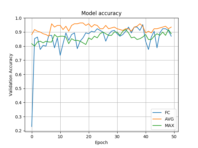
先看看准确度的比较:
再看看损失度的比较:

很明显,在InceptionV3模型下,FC、GAP和GMP都表现很好,但可以看出GAP的表现依旧最好,其准确度普遍在90%以上,而另两种的准确度在80~90%之间。
四、结论
从本实验看出,在数据集有限的情况下,采用经典模型进行迁移学习时,GMP表现不太稳定,FC层由于训练参数过多,更易导致过拟合现象的发生,而GAP则表现稳定,优于FC层。当然具体情况具体分析,我们拿到数据集后,可以在几种方式中多训练测试,以寻求最优解决方案。
深度学习基础系列(十)| Global Average Pooling是否可以替代全连接层?的更多相关文章
- 深度学习Keras框架笔记之Dense类(标准的一维全连接层)
深度学习Keras框架笔记之Dense类(标准的一维全连接层) 例: keras.layers.core.Dense(output_dim,init='glorot_uniform', activat ...
- 深度拾遗(06) - 1X1卷积/global average pooling
什么是1X1卷积 11的卷积就是对上一层的多个feature channels线性叠加,channel加权平均. 只不过这个组合系数恰好可以看成是一个11的卷积.这种表示的好处是,完全可以回到模型中其 ...
- 深度学习基础系列(九)| Dropout VS Batch Normalization? 是时候放弃Dropout了
Dropout是过去几年非常流行的正则化技术,可有效防止过拟合的发生.但从深度学习的发展趋势看,Batch Normalizaton(简称BN)正在逐步取代Dropout技术,特别是在卷积层.本文将首 ...
- 深度学习基础系列(五)| 深入理解交叉熵函数及其在tensorflow和keras中的实现
在统计学中,损失函数是一种衡量损失和错误(这种损失与“错误地”估计有关,如费用或者设备的损失)程度的函数.假设某样本的实际输出为a,而预计的输出为y,则y与a之间存在偏差,深度学习的目的即是通过不断地 ...
- 深度学习基础系列(一)| 一文看懂用kersa构建模型的各层含义(掌握输出尺寸和可训练参数数量的计算方法)
我们在学习成熟网络模型时,如VGG.Inception.Resnet等,往往面临的第一个问题便是这些模型的各层参数是如何设置的呢?另外,我们如果要设计自己的网路模型时,又该如何设置各层参数呢?如果模型 ...
- 深度学习基础系列(十一)| Keras中图像增强技术详解
在深度学习中,数据短缺是我们经常面临的一个问题,虽然现在有不少公开数据集,但跟大公司掌握的海量数据集相比,数量上仍然偏少,而某些特定领域的数据采集更是非常困难.根据之前的学习可知,数据量少带来的最直接 ...
- 深度学习基础系列(四)| 理解softmax函数
深度学习最终目的表现为解决分类或回归问题.在现实应用中,输出层我们大多采用softmax或sigmoid函数来输出分类概率值,其中二元分类可以应用sigmoid函数. 而在多元分类的问题中,我们默认采 ...
- 深度学习基础系列(七)| Batch Normalization
Batch Normalization(批量标准化,简称BN)是近些年来深度学习优化中一个重要的手段.BN能带来如下优点: 加速训练过程: 可以使用较大的学习率: 允许在深层网络中使用sigmoid这 ...
- 深度学习基础(十二)—— ReLU vs PReLU
从算法的命名上来说,PReLU 是对 ReLU 的进一步限制,事实上 PReLU(Parametric Rectified Linear Unit),也即 PReLU 是增加了参数修正的 ReLU. ...
随机推荐
- 浅谈ASP.net中的DataSet对象
在我们对数据库进行操作的时候,总是先把数据从数据库取出来,然后放到一个"容器"中,再通过这个"容器"取出数据显示在前台,而充当这种容器的角色中当属DataSet ...
- C++模拟OC的多重自动释放池
使用过OC的都知道,OC的引用计数机制用起来还比较方便.于是就仿照OC的形式搞了个C++引用计数. 支持多重自动释放池,每次autorelease都会放到栈顶的自动释放池中. 自动释放池也可以像变量一 ...
- 20155331 2016-2017-2 《Java程序设计》第6周学习总结
20155331 2016-2017-2 <Java程序设计>第6周学习总结 教材学习内容总结 输入/输出基础 很多实际的Java应用程序不是基于文本的控制台程序.尽管基于文本的程序作为教 ...
- 一个菜鸟的ASP.NET观光路线图
作为一个成长的"菜鸟".我的习惯是,每过一个阶段,都对自己的知识体系进行一次概括. 这篇博文是一个总结帖,我将把我的学到的东西,按照一定顺序串联在一起. ...
- element-UI 表单图片判空验证问题
本文地址:http://www.cnblogs.com/veinyin/p/8567167.html element-UI的表单验证似乎并没有覆盖到文件上传上面,当我们需要在表单里验证图片时,就会出 ...
- HDU 1176 排列2 全排列
解题报告:给出四个数,然后要你把这四个数组合成的各不相同的四位数按照从小到大的顺序输出来,然后如果最高位是0的话不能输出来,还有最高位是数字如果一样的话,则放在同一行输出. 本来是个比较简单的生成全排 ...
- 利用Django REST framework快速实现文件上传下载功能
安装包 pip install Pillow 设置 首先在settings.py中定义MEDIA_ROOT与MEDIA_URL.例如: MEDIA_ROOT = os.path.join(BASE_D ...
- Grunt、gulp、webpack、不要听着高大上你就上,试试Codekit?
下载地址:https://incident57.com/codekit/ 官方网站了解更多 要编译Less.Sass.Stylus, CoffeeScript, Typescript, Jade, H ...
- 差分约束系统专题 && 对差分约束系统的理解
具体能解决的问题: 求最长路,最短路,或者判断解是否存在. 在建边的时候: 一般是给你区间减法的关系,或者是这个点到另一个点的关系.如果给你的关系是除法的话,我们可以通过使用两边同时取log的方式,将 ...
- CentOS6.6 编译Redis报错:"Newer version of jemalloc required"
一.前言 不同系统同一个问题,可能解决方法不一样,也可能会遇到不同的问题,所以具体情况具体分析,我的系统是Centos6.6, 查看系统命令 cat /etc/issue 二.安装redis后编译报 ...