sklearn逻辑回归实战
题目要求
根据学生两门课的成绩和是否入学的数据,预测学生能否顺利入学:利用ex2data1.txt和ex2data2.txt中的数据,进行逻辑回归和预测。
数据放在最后边。
ex2data1.txt处理
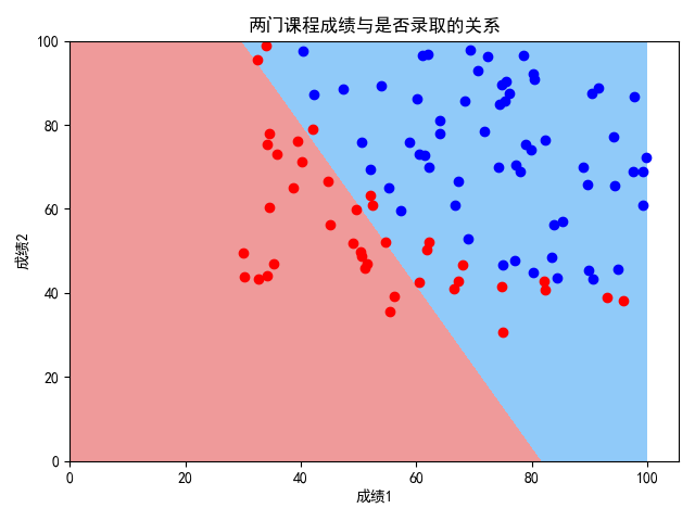
作散点图可知,决策大致符合线性关系,但还是有弯曲(非线性),用线性效果并不好,因此可用两种方案:方案一,无多项式特征;方案二,有多项式特征。
方案一:无多项式特征
对ex2data1.txt中的数据进行逻辑回归,无多项式特征
代码实现如下:
"""

    对ex2data1.txt中的数据进行逻辑回归(无多项式特征)

"""

from sklearn.model_selection import train_test_split

from matplotlib.colors import ListedColormap

from sklearn.linear_model import LogisticRegression

import numpy as np

import matplotlib.pyplot as plt

plt.rcParams['font.sans-serif'] = ['SimHei']  # 用来正常显示中文标签

plt.rcParams['axes.unicode_minus'] = False  # 用来正常显示负号

# 数据格式:成绩1,成绩2,是否被录取(1代表被录取,0代表未被录取)

# 函数(画决策边界)定义

def plot_decision_boundary(model, axis):

    x0, x1 = np.meshgrid(

        np.linspace(axis[0], axis[1], int((axis[1] - axis[0]) * 100)).reshape(-1, 1),

        np.linspace(axis[2], axis[3], int((axis[3] - axis[2]) * 100)).reshape(-1, 1),

    )

    X_new = np.c_[x0.ravel(), x1.ravel()]

    y_predict = model.predict(X_new)

    zz = y_predict.reshape(x0.shape)

    custom_cmap = ListedColormap(['#EF9A9A', '#FFF59D', '#90CAF9'])

    plt.contourf(x0, x1, zz, cmap=custom_cmap)

# 读取数据

data = np.loadtxt('ex2data1.txt', delimiter=',')

data_X = data[:, 0:2]

data_y = data[:, 2]

# 数据分割

X_train, X_test, y_train, y_test = train_test_split(data_X, data_y, random_state=666)

# 训练模型

log_reg = LogisticRegression()

log_reg.fit(X_train, y_train)

# 结果可视化

plot_decision_boundary(log_reg, axis=[0, 100, 0, 100])

plt.scatter(data_X[data_y == 0, 0], data_X[data_y == 0, 1], color='red')

plt.scatter(data_X[data_y == 1, 0], data_X[data_y == 1, 1], color='blue')

plt.xlabel('成绩1')

plt.ylabel('成绩2')

plt.title('两门课程成绩与是否录取的关系')

plt.show()

# 模型测试

print(log_reg.score(X_train, y_train))

print(log_reg.score(X_test, y_test))
输出结果如下:
0.8533333333333334

0.76
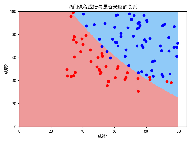
方案二:引入多项式特征
对ex2data1.txt中的数据进行逻辑回归,引入多项式特征。经调试,当degree为3时,耗费时间较长;当degree为2时,耗费时间可接受,效果与方案一相比好了很多
实现如下:
"""

    对ex2data1.txt中的数据进行逻辑回归(引入多项式特征)

"""

from sklearn.model_selection import train_test_split

from matplotlib.colors import ListedColormap

from sklearn.linear_model import LogisticRegression

import numpy as np

import matplotlib.pyplot as plt

from sklearn.preprocessing import PolynomialFeatures

from sklearn.pipeline import Pipeline

from sklearn.preprocessing import StandardScaler

plt.rcParams['font.sans-serif'] = ['SimHei']  # 用来正常显示中文标签

plt.rcParams['axes.unicode_minus'] = False  # 用来正常显示负号

# 数据格式:成绩1,成绩2,是否被录取(1代表被录取,0代表未被录取)

# 函数定义

def plot_decision_boundary(model, axis):

    x0, x1 = np.meshgrid(

        np.linspace(axis[0], axis[1], int((axis[1] - axis[0]) * 100)).reshape(-1, 1),

        np.linspace(axis[2], axis[3], int((axis[3] - axis[2]) * 100)).reshape(-1, 1),

    )

    X_new = np.c_[x0.ravel(), x1.ravel()]

    y_predict = model.predict(X_new)

    zz = y_predict.reshape(x0.shape)

    custom_cmap = ListedColormap(['#EF9A9A', '#FFF59D', '#90CAF9'])

    plt.contourf(x0, x1, zz, cmap=custom_cmap)

def PolynomialLogisticRegression(degree):

    return Pipeline([

        ('poly', PolynomialFeatures(degree=degree)),

        ('std_scaler', StandardScaler()),

        ('log_reg', LogisticRegression())

    ])

# 读取数据

data = np.loadtxt('ex2data1.txt', delimiter=',')

data_X = data[:, 0:2]

data_y = data[:, 2]

# 数据分割

X_train, X_test, y_train, y_test = train_test_split(data_X, data_y, random_state=666)

# 训练模型

poly_log_reg = PolynomialLogisticRegression(degree=2)

poly_log_reg.fit(X_train, y_train)

# 结果可视化

plot_decision_boundary(poly_log_reg, axis=[0, 100, 0, 100])

plt.scatter(data_X[data_y == 0, 0], data_X[data_y == 0, 1], color='red')

plt.scatter(data_X[data_y == 1, 0], data_X[data_y == 1, 1], color='blue')

plt.xlabel('成绩1')

plt.ylabel('成绩2')

plt.title('两门课程成绩与是否录取的关系')

plt.show()

# 模型测试

print(poly_log_reg.score(X_train, y_train))

print(poly_log_reg.score(X_test, y_test))
输出如下:
0.92

0.92
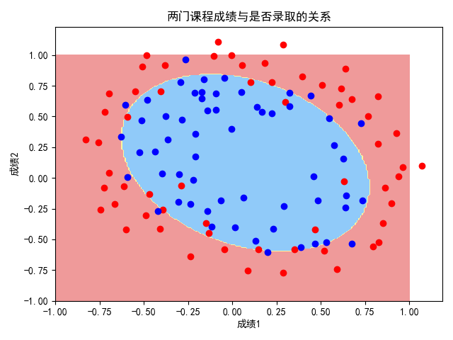
ex2data2.txt处理
作散点图可知,这组数据的决策边界绝对是非线性的,所以直接引入多项式特征对ex2data2.txt中的数据进行逻辑回归。
代码实现如下:
"""

    对ex2data2.txt中的数据进行逻辑回归(引入多项式特征)

"""

from sklearn.model_selection import train_test_split

from matplotlib.colors import ListedColormap

from sklearn.linear_model import LogisticRegression

import numpy as np

import matplotlib.pyplot as plt

from sklearn.preprocessing import PolynomialFeatures

from sklearn.pipeline import Pipeline

from sklearn.preprocessing import StandardScaler

plt.rcParams['font.sans-serif'] = ['SimHei']  # 用来正常显示中文标签

plt.rcParams['axes.unicode_minus'] = False  # 用来正常显示负号

# 数据格式:成绩1,成绩2,是否被录取(1代表被录取,0代表未被录取)

# 函数定义

def plot_decision_boundary(model, axis):

    x0, x1 = np.meshgrid(

        np.linspace(axis[0], axis[1], int((axis[1] - axis[0]) * 100)).reshape(-1, 1),

        np.linspace(axis[2], axis[3], int((axis[3] - axis[2]) * 100)).reshape(-1, 1),

    )

    X_new = np.c_[x0.ravel(), x1.ravel()]

    y_predict = model.predict(X_new)

    zz = y_predict.reshape(x0.shape)

    custom_cmap = ListedColormap(['#EF9A9A', '#FFF59D', '#90CAF9'])

    plt.contourf(x0, x1, zz, cmap=custom_cmap)

def PolynomialLogisticRegression(degree):

    return Pipeline([

        ('poly', PolynomialFeatures(degree=degree)),

        ('std_scaler', StandardScaler()),

        ('log_reg', LogisticRegression())

    ])

# 读取数据

data = np.loadtxt('ex2data2.txt', delimiter=',')

data_X = data[:, 0:2]

data_y = data[:, 2]

# 数据分割

X_train, X_test, y_train, y_test = train_test_split(data_X, data_y, random_state=666)

# 训练模型

poly_log_reg = PolynomialLogisticRegression(degree=2)

poly_log_reg.fit(X_train, y_train)

# 结果可视化

plot_decision_boundary(poly_log_reg, axis=[-1, 1, -1, 1])

plt.scatter(data_X[data_y == 0, 0], data_X[data_y == 0, 1], color='red')

plt.scatter(data_X[data_y == 1, 0], data_X[data_y == 1, 1], color='blue')

plt.xlabel('成绩1')

plt.ylabel('成绩2')

plt.title('两门课程成绩与是否录取的关系')

plt.show()

# 模型测试

print(poly_log_reg.score(X_train, y_train))

print(poly_log_reg.score(X_test, y_test))
输出结果如下:
由图可知,分类结果较好。
0.7954545454545454

0.9
两份数据
ex2data1.txt
34.62365962451697,78.0246928153624,0

30.28671076822607,43.89499752400101,0

35.84740876993872,72.90219802708364,0

60.18259938620976,86.30855209546826,1

79.0327360507101,75.3443764369103,1

45.08327747668339,56.3163717815305,0

61.10666453684766,96.51142588489624,1

75.02474556738889,46.55401354116538,1

76.09878670226257,87.42056971926803,1

84.43281996120035,43.53339331072109,1

95.86155507093572,38.22527805795094,0

75.01365838958247,30.60326323428011,0

82.30705337399482,76.48196330235604,1

69.36458875970939,97.71869196188608,1

39.53833914367223,76.03681085115882,0

53.9710521485623,89.20735013750205,1

69.07014406283025,52.74046973016765,1

67.94685547711617,46.67857410673128,0

70.66150955499435,92.92713789364831,1

76.97878372747498,47.57596364975532,1

67.37202754570876,42.83843832029179,0

89.67677575072079,65.79936592745237,1

50.534788289883,48.85581152764205,0

34.21206097786789,44.20952859866288,0

77.9240914545704,68.9723599933059,1

62.27101367004632,69.95445795447587,1

80.1901807509566,44.82162893218353,1

93.114388797442,38.80067033713209,0

61.83020602312595,50.25610789244621,0

38.78580379679423,64.99568095539578,0

61.379289447425,72.80788731317097,1

85.40451939411645,57.05198397627122,1

52.10797973193984,63.12762376881715,0

52.04540476831827,69.43286012045222,1

40.23689373545111,71.16774802184875,0

54.63510555424817,52.21388588061123,0

33.91550010906887,98.86943574220611,0

64.17698887494485,80.90806058670817,1

74.78925295941542,41.57341522824434,0

34.1836400264419,75.2377203360134,0

83.90239366249155,56.30804621605327,1

51.54772026906181,46.85629026349976,0

94.44336776917852,65.56892160559052,1

82.36875375713919,40.61825515970618,0

51.04775177128865,45.82270145776001,0

62.22267576120188,52.06099194836679,0

77.19303492601364,70.45820000180959,1

97.77159928000232,86.7278223300282,1

62.07306379667647,96.76882412413983,1

91.56497449807442,88.69629254546599,1

79.94481794066932,74.16311935043758,1

99.2725269292572,60.99903099844988,1

90.54671411399852,43.39060180650027,1

34.52451385320009,60.39634245837173,0

50.2864961189907,49.80453881323059,0

49.58667721632031,59.80895099453265,0

97.64563396007767,68.86157272420604,1

32.57720016809309,95.59854761387875,0

74.24869136721598,69.82457122657193,1

71.79646205863379,78.45356224515052,1

75.3956114656803,85.75993667331619,1

35.28611281526193,47.02051394723416,0

56.25381749711624,39.26147251058019,0

30.05882244669796,49.59297386723685,0

44.66826172480893,66.45008614558913,0

66.56089447242954,41.09209807936973,0

40.45755098375164,97.53518548909936,1

49.07256321908844,51.88321182073966,0

80.27957401466998,92.11606081344084,1

66.74671856944039,60.99139402740988,1

32.72283304060323,43.30717306430063,0

64.0393204150601,78.03168802018232,1

72.34649422579923,96.22759296761404,1

60.45788573918959,73.09499809758037,1

58.84095621726802,75.85844831279042,1

99.82785779692128,72.36925193383885,1

47.26426910848174,88.47586499559782,1

50.45815980285988,75.80985952982456,1

60.45555629271532,42.50840943572217,0

82.22666157785568,42.71987853716458,0

88.9138964166533,69.80378889835472,1

94.83450672430196,45.69430680250754,1

67.31925746917527,66.58935317747915,1

57.23870631569862,59.51428198012956,1

80.36675600171273,90.96014789746954,1

68.46852178591112,85.59430710452014,1

42.0754545384731,78.84478600148043,0

75.47770200533905,90.42453899753964,1

78.63542434898018,96.64742716885644,1

52.34800398794107,60.76950525602592,0

94.09433112516793,77.15910509073893,1

90.44855097096364,87.50879176484702,1

55.48216114069585,35.57070347228866,0

74.49269241843041,84.84513684930135,1

89.84580670720979,45.35828361091658,1

83.48916274498238,48.38028579728175,1

42.2617008099817,87.10385094025457,1

99.31500880510394,68.77540947206617,1

55.34001756003703,64.9319380069486,1

74.77589300092767,89.52981289513276,1
ex2data2.txt
0.051267,0.69956,1

-0.092742,0.68494,1

-0.21371,0.69225,1

-0.375,0.50219,1

-0.51325,0.46564,1

-0.52477,0.2098,1

-0.39804,0.034357,1

-0.30588,-0.19225,1

0.016705,-0.40424,1

0.13191,-0.51389,1

0.38537,-0.56506,1

0.52938,-0.5212,1

0.63882,-0.24342,1

0.73675,-0.18494,1

0.54666,0.48757,1

0.322,0.5826,1

0.16647,0.53874,1

-0.046659,0.81652,1

-0.17339,0.69956,1

-0.47869,0.63377,1

-0.60541,0.59722,1

-0.62846,0.33406,1

-0.59389,0.005117,1

-0.42108,-0.27266,1

-0.11578,-0.39693,1

0.20104,-0.60161,1

0.46601,-0.53582,1

0.67339,-0.53582,1

-0.13882,0.54605,1

-0.29435,0.77997,1

-0.26555,0.96272,1

-0.16187,0.8019,1

-0.17339,0.64839,1

-0.28283,0.47295,1

-0.36348,0.31213,1

-0.30012,0.027047,1

-0.23675,-0.21418,1

-0.06394,-0.18494,1

0.062788,-0.16301,1

0.22984,-0.41155,1

0.2932,-0.2288,1

0.48329,-0.18494,1

0.64459,-0.14108,1

0.46025,0.012427,1

0.6273,0.15863,1

0.57546,0.26827,1

0.72523,0.44371,1

0.22408,0.52412,1

0.44297,0.67032,1

0.322,0.69225,1

0.13767,0.57529,1

-0.0063364,0.39985,1

-0.092742,0.55336,1

-0.20795,0.35599,1

-0.20795,0.17325,1

-0.43836,0.21711,1

-0.21947,-0.016813,1

-0.13882,-0.27266,1

0.18376,0.93348,0

0.22408,0.77997,0

0.29896,0.61915,0

0.50634,0.75804,0

0.61578,0.7288,0

0.60426,0.59722,0

0.76555,0.50219,0

0.92684,0.3633,0

0.82316,0.27558,0

0.96141,0.085526,0

0.93836,0.012427,0

0.86348,-0.082602,0

0.89804,-0.20687,0

0.85196,-0.36769,0

0.82892,-0.5212,0

0.79435,-0.55775,0

0.59274,-0.7405,0

0.51786,-0.5943,0

0.46601,-0.41886,0

0.35081,-0.57968,0

0.28744,-0.76974,0

0.085829,-0.75512,0

0.14919,-0.57968,0

-0.13306,-0.4481,0

-0.40956,-0.41155,0

-0.39228,-0.25804,0

-0.74366,-0.25804,0

-0.69758,0.041667,0

-0.75518,0.2902,0

-0.69758,0.68494,0

-0.4038,0.70687,0

-0.38076,0.91886,0

-0.50749,0.90424,0

-0.54781,0.70687,0

0.10311,0.77997,0

0.057028,0.91886,0

-0.10426,0.99196,0

-0.081221,1.1089,0

0.28744,1.087,0

0.39689,0.82383,0

0.63882,0.88962,0

0.82316,0.66301,0

0.67339,0.64108,0

1.0709,0.10015,0

-0.046659,-0.57968,0

-0.23675,-0.63816,0

-0.15035,-0.36769,0

-0.49021,-0.3019,0

-0.46717,-0.13377,0

-0.28859,-0.060673,0

-0.61118,-0.067982,0

-0.66302,-0.21418,0

-0.59965,-0.41886,0

-0.72638,-0.082602,0

-0.83007,0.31213,0

-0.72062,0.53874,0

-0.59389,0.49488,0

-0.48445,0.99927,0

-0.0063364,0.99927,0

0.63265,-0.030612,0
作者:@臭咸鱼
转载请注明出处:https://www.cnblogs.com/chouxianyu/
欢迎讨论和交流!
sklearn逻辑回归实战的更多相关文章
- 通俗地说逻辑回归【Logistic regression】算法(二)sklearn逻辑回归实战
前情提要: 通俗地说逻辑回归[Logistic regression]算法(一) 逻辑回归模型原理介绍 上一篇主要介绍了逻辑回归中,相对理论化的知识,这次主要是对上篇做一点点补充,以及介绍sklear ...
- sklearn逻辑回归(Logistic Regression,LR)调参指南
python信用评分卡建模(附代码,博主录制) https://study.163.com/course/introduction.htm?courseId=1005214003&utm_ca ...
- sklearn逻辑回归
sklearn逻辑回归 logistics回归名字虽然叫回归,但实际是用回归方法解决分类的问题,其形式简洁明了,训练的模型参数还有实际的解释意义,因此在机器学习中非常常见. 理论部分 设数据集有n个独 ...
- sklearn逻辑回归(Logistic Regression)类库总结
class sklearn.linear_model.LogisticRegression(penalty=’l2’, dual=False, tol=0.0001, C=1.0, fit_inter ...
- sklearn逻辑回归库函数直接拟合数据
from sklearn import model_selection from sklearn.linear_model import LogisticRegression from sklearn ...
- 机器学习入门-概率阈值的逻辑回归对准确度和召回率的影响 lr.predict_proba(获得预测样本的概率值)
1.lr.predict_proba(under_text_x) 获得的是正负的概率值 在sklearn逻辑回归的计算过程中,使用的是大于0.5的是正值,小于0.5的是负值,我们使用使用不同的概率结 ...
- 逻辑回归原理_挑战者飞船事故和乳腺癌案例_Python和R_信用评分卡(AAA推荐)
sklearn实战-乳腺癌细胞数据挖掘(博客主亲自录制视频教程) https://study.163.com/course/introduction.htm?courseId=1005269003&a ...
- 逻辑回归--美国挑战者号飞船事故_同盾分数与多头借贷Python建模实战
python信用评分卡(附代码,博主录制) https://study.163.com/course/introduction.htm?courseId=1005214003&utm_camp ...
- 机器学习_线性回归和逻辑回归_案例实战:Python实现逻辑回归与梯度下降策略_项目实战:使用逻辑回归判断信用卡欺诈检测
线性回归: 注:为偏置项,这一项的x的值假设为[1,1,1,1,1....] 注:为使似然函数越大,则需要最小二乘法函数越小越好 线性回归中为什么选用平方和作为误差函数?假设模型结果与测量值 误差满足 ...
随机推荐
- Egret入门学习日记 --- 第十五篇(书中 6.1~6.9节 内容)
第十五篇(书中 6.1~6.9节 内容) 好的,昨天完成了第五章. 今天来看第六章. 总结重点: 1.如何对组件进行分组? 跟着做: 重点1:如何对组件进行分组? 首先,选中你想要组合的组件. 然后点 ...
- clog就用clog的后缀名
/tmp/log/shuanggou.clog /tmp/log/shuanggou.log /tmp/log/shuanggou_success.log /tmp/log/shuanggou_err ...
- 【Linux内核】编译与配置内核(x86)
[Linux内核]编译与配置内核(x86) https://www.cnblogs.com/jamesharden/p/6414736.html
- kubernetes 部署ingress
kubernetes Ingess 是有2部分组成,Ingress Controller 和Ingress服务组成,常用的Ingress Controller 是ingress-nginx,工作的原理 ...
- LC 173. Binary Search Tree Iterator
题目描述 Implement an iterator over a binary search tree (BST). Your iterator will be initialized with t ...
- 利用sort对结构体进行排序
我定义了一个学生类型的结构体来演示sort排序对结构体排序的用法 具体用法看代码 #include<iostream> #include<string> #include< ...
- go 结构的方法2
你可以对包中的 任意 类型定义任意方法,而不仅仅是针对结构体. 但是,不能对来自其他包的类型或基础类型定义方法. package main import ( "fmt" ...
- 微信小程序页面滚动到指定位置
页面上有一个元素或者组件,id 为 comment 则: var me = this; var query = wx.createSelectorQuery().in(me); query.selec ...
- 网络知识(1)TCP/IP五层结构
图1 数据流向图 1,网络基础 1.1 发展 古代:①烽火狼烟最为原始的0-1单bit信息传递:②飞鸽传书.驰道快马通信,多字节通信: 近代:①轮船信号灯:②无线电报[摩尔斯码]: 现代:①有线模拟通 ...
- 50道高级sql练习题;大大提高自己的sql能力(附具体的sql)
问题及描述:--1.学生表Student(SID,Sname,Sage,Ssex) --SID 学生编号,Sname 学生姓名,Sage 出生年月,Ssex 学生性别--2.课程表Course(CID ...