SciTech-Mathmatics-Sinusoids正弦波/Harmonics(谐波) + FrequenciesSynthesis(频率合成) + Fourier Series(傅里叶级数):PeriodicalFunctions + (Discrete)FourierTransform:AllFunctions + Spectral Analysis

几何角度看，Fourier Series(傅立叶级数) 其实非常容易理解:

1. 每一组\((\cos(2\pi n f t),\ \sin(2\pi n f t))\)三角函数都可看作决定一“谐波空间”的 \(x\) 轴与 \(y\) 轴;
   
   Time-domain 的信号, 是用 Freq.-domain 的 N 个独立空间的谐波合成;
   
   每一个“谐波空间”, 都是一对可配置\(( freq.,\ magnitude,\ phase)\)的三角函数(cos/sin);
   
   每一个“谐波空间”, 都有三个坐标轴: \((1, \cos(2\pi n f t), \sin(2\pi n f t))\):
   
   \(\large \begin{array}{ll} \\ x(t) &= \frac{a_0}{2} + \sum_{n=1}^{\infty} {[\ a_{n} \cos(2\pi n f t) + b_{n}\sin(2\pi n f t) \ ]} \\
   & \frac{a_0}{2} \longrightarrow 分解到基函数1(常数函数)对应的坐标轴上的坐标 \\
   & a_n \longrightarrow 分解到 基函数 \cos(2\pi n f t) 对应的坐标轴上的坐标 \\
   & b_n \longrightarrow 分解到 基函数 \sin(2\pi n f t) 对应的坐标轴上的坐标 \\
   \end{array}\)

   \(\large \begin{array}{ll} \\ x(t) &= \int_{n=-\infty}^{+\infty}{S_n \cdot e^{i\frac{2\pi n t}{T}}} dt \\
   S_n &= \frac{1}{T} \int_{t_0}^{t_0+T}{ x(t) \cdot e^{-i\frac{2\pi n t}{T}}} dt \\
   & S_n: 分解到 正交基函数(复函数)\ e^{i 2\pi n f t}\ 坐标轴上的坐标 \\
   \\
   when & T \rightarrow \infty, \bf{即频域 谐波组频点 无穷多, 就变成“连续的频带”} \\
   F(\omega) &= \frac{1}{2\pi} \int_{-\infty}^{+\infty}{x(t) \cdot e^{-i \omega t}} dt \\
   & \omega: 代表频率 \\
   \\ \end{array}\)

2. 合成的 \(\large X(t)\) 周期为 \(T = \frac{1}{f}\),
   
   是因为其 \(k\) 个Frequency Components(频率成分) 的 周期的最小公倍数为 T;
   
   这些 Harmonics(Frequency Components) 谐波任意“加减”组合, 周期最小公倍数为 T.
   
   下文 “Preliminaries.3. Frequency Components) for Synthesis” 有述;

3. 内积(inner product of vectors) 与 分解;

   • 向量的内积, 在有限维向量空间, 两个向量的内积:
     
     \(\large \begin{array}{rl} \overrightarrow{u} \cdot \overrightarrow{v} &= x_1 x_2 + y_1 y_2 \\
     where & \overrightarrow{u} = (x_1, y_1),\ \overrightarrow{v} = (x_2, y_2) \\
     \end{array}\)

   • 函数的内积, 在无限维函数空间, 两个函数(连续)的内积(内积要重新定义,用到积分):
     
     \(\large \begin{array}{rl} <f, g> &= \int_{t_0}^{t_0 + T}{f(t)g(t)} dt \end{array}\)

   • 离散向量分解:
     
     将向量 \(\overrightarrow{u}\) 分解到 两个"正交向量" \(\overrightarrow{v_1}\) 与 \(\overrightarrow{v_2}\)上:
     
     假设在(\(\overrightarrow{v_1}\), \(\overrightarrow{v_2}\))两坐标轴上坐标为(\(c_1\), \(c_2\)), 则有:
     
     \(\large \begin{array}{ll} \ & \\
     & \overrightarrow{u} = c_1 \overrightarrow{v_1} + c_2 \overrightarrow{v_2} \\
     & 分解出的坐标(c_1, c_2)分别为: \\
     & c_1 = \frac{\overrightarrow{u} \cdot \overrightarrow{v_1}}{\overrightarrow{v_1} \cdot \overrightarrow{v_1}},\ c_2 = \frac{\overrightarrow{u} \cdot \overrightarrow{v_2}}{\overrightarrow{v_2} \cdot \overrightarrow{v_2}} \\
     \\ \end{array}\)

   • 连续向量分解:
     
     将连续向量函数 \(\overrightarrow{x(t)}\) 分解到 两个"正交基函数" \(\overrightarrow{\cos(2\pi n f t)}\) 与 \(\overrightarrow{\sin(2\pi n f t)}\)上:
     
     要将以上向量分解公式,由 有限维的向量空间 扩展到 无限维的函数空间;
     
     要将内积由 有限维的向量空间 扩展到 无限维的函数空间,
     
     并且, 要将每个三角函数(cos/sin)都看作一个“独立的坐标轴”,
     
     用到 上文的 “函数的内积” 积分公式.
     
     但是为方便高效, 最好用 \(Euler's\ Equation\) 将$cos/sin转换为:
     
     \(\large \begin{array}{ll} \because & s_n &= \frac{1}{T} \int_{t_0}^{t_0 + T}{x(t) \cdot e^{-i2\pi n f t}} dt \\
     & T &= \infty \\
     \therefore & F(\omega) &= \frac{1}{2\pi} \int_{-\infty}^{+\infty}{x(t) \cdot e^{-i \omega t}} dt \\
     \\ \end{array}\)

4. 向量的正交与分解: 投影到正交的一堆向量为基的空间;
   
   之所以选择分解到 \(f(\theta) = \cos \theta\) 与 \(f(\theta) = \sin \theta\), 是因为这是“一对正交基函数”,
   
   而且在任意时刻 \(t_0\) 开始, 时长 \(2\pi\) 的 \(\sin{x} \cos{x}\) 信号的积分都是\(0\):
   
   \(\large \begin{array}{rl} <sin, cos> &= \int_{ t_0}^{t_0 + 2\pi}{\sin{x} \cos{x}} dx = 0 \end{array}\)

   类比: 就像\(XOY\)平面的\(X轴\) 与 \(Y轴\) 是正交的,
   
   因此\(XOY\)平面上任何一点, 可用其分别在\(X轴\) 与 \(Y轴\)上的投影作为(x,y)坐标;

   向量正交: 对于 \(XOY\)平面上两个向量 \(\overrightarrow{u} = (x_1, y_1),\ \overrightarrow{v} = (x_2, y_2)\),
   
   如果它们的内积为0, 夹角为\(90^{\circ}\), 则称这两个向量点是“正交的”, 即 :
   
   \(\large \begin{array}{rl} \overrightarrow{u} \cdot \overrightarrow{v} = x_1 x_2 + y_1 y_2 = 0 \\ \end{array}\)

   函数正交: 余弦函数$ \cos \theta $ 与 正弦函数$ \sin \theta $,
   
   可看作 无限维的 Hilbert 空间 的 无限维向量, 向量的各个“元”是连续区间的“函数值”;
   
   无限维空间的向量内积需要用到积分重新定义为“两个连续函数的函数值先相乘后积分”:
   
   \(\large \begin{array}{rl} <f, g> &= \int_{x_0}^{x_0 + T}{f(x)g(x)} dx \\
   <sin, cos> &= \int_{t_0}^{t_0 + 2\pi}{\sin{t} \cos{t}} dt = 0
   \end{array}\)

5. 分解 Time-domain 信号到 Frequency-domain,
   
   总体思路上, 与“Taylor Series(泰勒级数)拟合任意N阶可导函数”类似:

   • Taylor Series 是以无限项 $\large a_j (x-x_0)^j $(带可调参数的幂函数) 合成任意的 \(\large f(x)\);
     
     确定系数 \(\large a_j\) 与 \(\large x_0\) 是用 \(\large f'(x),\ f''(x), f^{3}(x),\ ...\ ,\ , f^{n}(x)\) 无限高阶导数进行拟合与误差估计;

   • Fourier Series 是以无限项 \(\large [\ a_{n} \cos(2\pi n f t) + b_{n}\sin(2\pi n f t) \ ]\)(可配置系数的sin正弦信号发生器);
     
     确定系数 \(a_n\) 与 \(b_n\) 是用 积分/复数 运算 进行拟合与误差估计;

   实际上, 把 Time-domain 的 Signal 函数 \(X(t)\) 分解/投影到 Frequency-domain 的多个“平面”(sin信号发生器):

   • 每个“平面”有 一对“正交基函数”(cos/sin), 实现上是一组(\(N\)个)“可配置系数”的sin信号发生器(谐波信号轮);
     
     每个“sin正弦信号轮”的用:

     • 半径(Radius)表示\(magnitude\)系数,
     • 用起始的距0弧度的bias量表示\(phase\)系数,
     • 以配置的常数的转动频率周期转动(产生信号)表示 Harmonic(\(\large nf_0\)) 固定的谐波频率;

     通过这一组(\(N\)个)“sin信号轮”以配置好的\((magnitude,\ phase,\ harmonic)\)同时转动(产生信号),
     
     可以合成任意的周期函数; 谐波信号轮个数越多(\(N\)越大)越精准;

   • 参数 \((a_j, b_j)\) 可以导出\((magnitude,\ phase)\), 因为 \(frequency\)这个系数,
     
     总是 Harmonic(谐波频点, “基频\(\large f\)”的自然数倍), 所以可视为可变的常数;
     
     因此实际最需要确定的系数\((magnitude,\ phase)\)用 \((a_j, b_j)\) 导出就足够;
     
     Sampling在任意时刻\(\large t_0\), 最短采集(\(\bf{T_0 = \frac{1}{f_0}}\)(the fundamental period)$时长就足够;

6. 既可以选用 sin 系列的正弦函数, 也可以选用 cos系列的余弦函数;
   
   之所以选用 cos 与 sin 两个函数作为“基函数”:

   • 因为 cos 与 sin 这一对“基函数”正交.
   • cos 与 sin 可以非常好的与 Complex Space 转换;
   • cos 与 sin 可以用 Euler's Equation $\large e^{i\theta} = \cos\theta + i \sin\theta $ 进行变换计算;
   • cos 与 sin 在 实现、转换、变换 以及 实际应用 时非常方便实现.
     
     \(\large cos\theta\) 可用 \(\large sin{(\theta - \frac{\pi}{2})}\) 合成(即phase左移\(\large \frac{\pi}{2}\));
     
     实现上, 只要做好一种可配置(freq., magnitude, phase)的 sin正弦信号发生器就可规模化量产;
   • 总之优点众多.

Preliminaries

1. Periodic signals:

   At least to begin, we’ll mainly be concerned with signals that are periodic.
   
   Informally, a periodic signal is one that repeats, over and over, forever. To be more precise:
   
   A signal \(x(t)\) is said to be periodic if there exists some number \(T\),
   
   \(\large \begin{array}{lll} \text{such that} & \\
   x(t) &=& x(t+T) \text{ , for all } t \\
   & & \ T:\ \mathbf{\text{the period of the signal} } \\
   & & \ \mathbf{smallest\ } T:\ \mathbf{\text{the fundamental period}} \\
   \end{array}\).

2. Sinusoids:

   Precisely what do we mean by a sinusoid? The term “sinusoid” means a sine wave,
   
   but we don’t just mean the standard \(\sin(t)\). To enable our analysis,
   
   we want to be able to work sine waves of different \(heights\), \(widths\) and \(phases\).
   
   So, to us, a single sinusoid means a function of the form
   
   \(\large \begin{array}{lll} \\
   \ \ \ \ & x(t) &= A& \sin(2\pi f t + \phi) \\
   \text{for some} & & \\
   & & A &its\ amplitude \\
   & & f &its\ frequency,\ period\ T = \frac{1}{f} \\
   & & \phi &its\ phase \\
   \end{array}\),

3. Frequency Components for Synthesis:

   \(\begin{array}{rlll} GIVING& &&& \\
   x_{1}(t) &=& A_1 \sin (1 \times (2\pi f t + \phi ) ) \ ,\ \text{ freq.: } \ f\ ,\ \text{ amplitude:} A_1\ ,\ \text{ phase:} \ \phi \\
   x_{2}(t) &=& A_2 \sin (2 \times (2\pi f t + \phi) ) \ ,\ \text{ freq.: } 2f\ ,\ \text{ amplitude:} A_2\ ,\ \text{ phase:} 2\phi \\
   x_{3}(t) &=& A_3 \sin (3 \times (2\pi f t + \phi) ) \ ,\ \text{ freq.: } 3f\ ,\ \text{ amplitude:} A_3\ ,\ \text{ phase:} 3\phi \\
   ...& & \\
   x_{k}(t) &=& A_k \sin (k \times (2\pi f t + \phi) ) \ ,\ \text{ freq.: } nf\ ,\ \text{ amplitude:} A_k\ ,\ \text{ phase:} k\phi \\
   \\
   X(t) &=& \sum_{n=1}^{k} x_{n}(t) & \\
   &=& \sum_{n=1}^{k} { A_{n} \sin[\ n(2\pi f t + \phi)\ ] } & \\
   \\ \end{array}\)
   
   \(\text{ THEN the }\mathbf{period}\ of\ X(t)\text{ is } T = \frac{1}{f}, \text{SINCE}\)
   
   \(\begin{array}{rlll} \\
   \ \ period(x_{1}) &= T &= \frac{1}{f}, \\
   \ \ period(x_{2}) &= \frac{T}{2} &= \frac{1}{2f}, \\
   \ \ period(x_{3}) &= \frac{T}{3} &= \frac{1}{3f}, \\
   \ \ &... & \\
   \ \ period(x_{k}) &= \frac{T}{k} &= \frac{1}{kf}, \\
   \\ \end{array}\)

4. Harmonics/Sinusoids:

   The sinusoidal terms are often called \(\mathbf{harmonics}\), a term borrowed from music.
   
   The harmonics will have frequencies \(f\ ,\ 2f\ ,\ 3f\ ,\ 4f\) and so on.
   
   We also call each \(harmonic\), \(A_n \sin(2\pi n f t + \phi n)\), the \(\mathbf{frequency\ component}\) of \(x(t)\) at frequency \(n f\).
   
   For example, if \(f = 10Hz\), we call the \(harmonic\) for which
   
   \(n = 3\) the “\(30Hz\ component\)”, reflecting that
   
   in this case \(\sin(2\pi n f t+\phi n)\) is a sinusoid of frequency \(30Hz\)

5. Frequency-domain and Time-domain Representation:

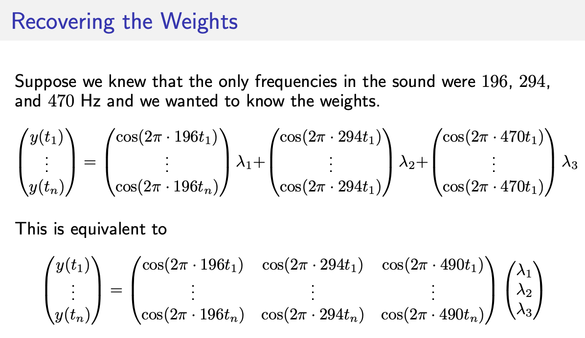
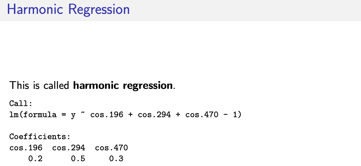
   • the frequency-domain representation of the periodic signal:
     
     represent a signal using the magnitudes and phases in its Fourier series.
     
     We often plot the magnitudes in the Fourier series,
     
     using a stem graph and labeling the frequency axis by frequency.
     
     In this sense, this representation is a function of frequency.
   • the time-domain representation of the signal:
     
     represent a periodic signal as a function of time in its Fourier series.
   • Example:
     
     

The Fourier Series:

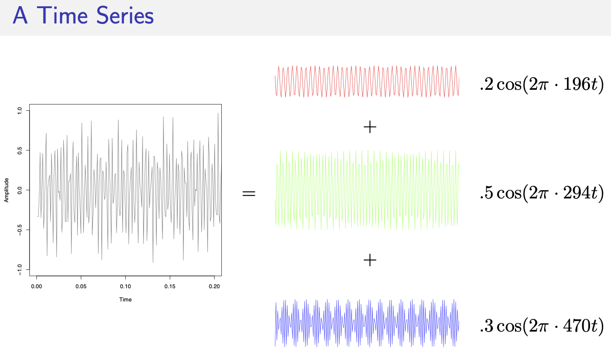
• Joseph Fourier’s idea was to express periodic signals as a sum of sinusoids.
• Theorem.

  • If \(\mathbf{ x(t) }\) is a \(\text{ well-behaved periodic signal }\) with \(\large \mathbf{ period\ T}\),

    $\large \text{ We call }\mathbf{\ following\ sum } \ the\ \mathbf{\ Fourier\ series\ of\ }x(t) $
    
    \(\large \begin{array}{ll} x(t) &= \begin{equation} A_0 + \sum_{n=1}^{\infty} { A_{n} \sin(2\pi n f t + n\phi) } \tag{1F} \end{equation} \\
    & \mathbf{ frequency }: f = 1/T, \\
    & \mathbf{ magnitudes }: A_i\ ,\ i \in [\ 1, +\infty\ ] \\
    & \mathbf{ phases } \phi_i\ ,\ i \in [\ 1, +\infty\ ] \\
    \\ \end{array}\)
    
    Another fact relating to Fourier series is that:
    
    the $magnitudes\ A_0\ ,\ A_1\ ,\ A_2\ ,\ ... $ and $phases\ \phi_1\ ,\ \phi_2\ ,\ ... $
    
    in above equation uniquely determine \(x(t)\). That is, if we can find these
    
    $ magnitudes $ and \(phases\) corresponding to a periodic signal \(x(t)\),
    
    then, in effect, we have another way of describing \(x(t)\).

  • \(\large \text{ Another useful form of Fourier series of }x(t)\)
    
    \(\large \begin{array}{ll} x(t) &= \begin{equation} \frac{a_0}{2} + \sum_{n=1}^{\infty} {[\ a_{n} \cos(2\pi n f t) + b_{n}\sin(2\pi n f t) \ ]} \tag{2F} \end{equation} \\
    & a_{0} = 2 A_0\ , \\
    & a_{n} = A_{n}\cos{(n\phi)}\ ,\ b_{n} = A_{n}\sin{(n\phi)}\ , \\
    & (a_{n})^{2} + (b_{n})^{2} = (A_{n})^{2}\ \\
    & \text{ above } \mathbf{coefficients}\text{ can then be found, } \\
    & \text{ using the following integrals, where }T = \frac{1}{f}: \\
    & a_n = \frac{2}{T} \int_{0}^{T}{x(t)\cos(2\pi n f t)} dt \, \\
    & b_n = \frac{2}{T} \int_{0}^{T}{x(t)\sin(2\pi n f t)} dt \\
    &\text{ and }a_0,\ a_1,\ a_2,\ . . .\text{ and }b_1,\ b_2,\ . . .\ \\
    &\text{ can be converted to }magnitudes\text{ and }phases,\ \\
    &\text{ to fit above form (1F) }. \\
    \\ \end{array}\)

    \(\large \text{ Proof of form (1F) and form (2F) are the same }\)
    
    \(\large \begin{array}{lll} \\
    & \because & \sin(X + Y) = \sin{X} \cos{Y} + \cos{X} sin{Y} \\
    & \therefore & \sin(2\pi n f t + n\phi) = \sin{(2\pi n f t)} \cos{(n\phi)} + \cos{(2\pi n f t)} sin{(n\phi)} \\
    & x(t) &= A_0 + \sum_{n=1}^{\infty} { A_{n} \sin(2\pi n f t + n\phi) } \\
    & &= A_0 + \sum_{n=1}^{\infty} { (A_{n}\cos{(n\phi)}) \sin{(2\pi n f t)} + (A_{n}\sin{(n\phi)}) \cos{(2\pi n f t)}\ ] } \\
    & & = \frac{a_0}{2} + \sum_{n=1}^{\infty} {[\ a_{n} \cos(2\pi n f t) + b_{n}\sin(2\pi n f t) \ ]} \\
    \\ \end{array}\)

  • \(\large \text{ Complex form of Fourier series of }x(t)\)
    
    \(\large \begin{array}{lll} \because e^{i\theta} &= \cos\theta + i\sin\theta ,\text{ the Euler's Equation}\\
    \therefore e^{i2 \pi n f t} &= \cos{(2 \pi n f t)} + i\sin{(2 \pi n f t)} \\
    x(t) &= \frac{a_0}{2} + \sum_{n=1}^{\infty} {[\ a_{n} \cos(2\pi n f t) + b_{n}\sin(2\pi n f t) \ ]} \\
    &= \frac{1}{T} \int_{t_0}^{t_0 + T}{x(t) \cdot e^{-i2\pi n f t}} dt \\
    \\ \end{array}\)

    \(\large \begin{array}{ll} \because & S_n &= \frac{1}{T} \int_{t_0}^{t_0 + T}{x(t) \cdot e^{-i2\pi n f t}} dt \\
    & T &= \infty \\
    \therefore & F(\omega) &= \frac{1}{2\pi} \int_{-\infty}^{+\infty}{x(t) \cdot e^{-i \omega t}} dt \\
    \\ \end{array}\)

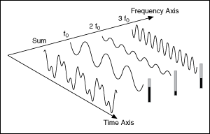
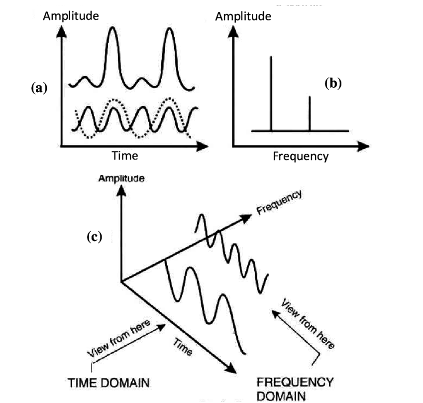
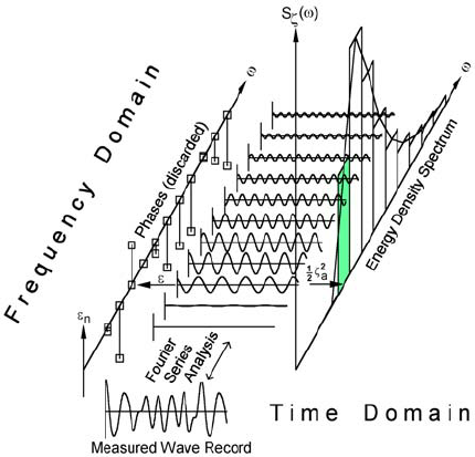
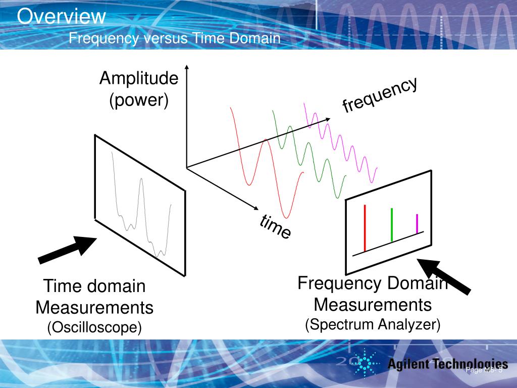
Time Domain + Frequency Domain

and Fourier Transforms @ Princeton University:

Fourier Series: Periodical Functions

Fourier Transform: All Functions

Frequency Domain and Fourier Transforms @ Princeton University:

https://www.princeton.edu/~cuff/ele201/kulkarni_text/frequency.pdf

Signals and the frequency domain

ENGR 40M lecture notes — July 31, 2017 Chuan-Zheng Lee, Stanford University

https://web.stanford.edu/class/archive/engr/engr40m.1178/slides/signals.pdf

https://www.mathworks.com/help/signal/ug/extract-regions-of-interest-from-whale-song.html

https://web.stanford.edu/class/stats253/lectures_2014/lect7.pdf

https://web.stanford.edu/class/stats253/lectures_2014/

https://resources.pcb.cadence.com/blog/2020-time-domain-analysis-vs-frequency-domain-analysis-a-guide-and-comparison

• Time Domain and Frequency Domain:
  • Illustrations:
    
    | | | |
    
    | ---- | ---- | ---- |
    
    | | | |

• Application: The role of ECoG magnitude and phase in decoding position, velocity, and acceleration during continuous motor behavior
  
  

• Frequency Domain and Fourier Transforms @ Princeton University:
  
  https://www.princeton.edu/~cuff/ele201/kulkarni_text/frequency.pdf
  
  

• Signals @ WEB.stanford.edu
  
  https://web.stanford.edu/class/archive/engr/engr40m.1178/slides/signals.pdf

• https://web.stanford.edu/class/stats253/lectures_2014/lect7.pdf

The Frequency Domain

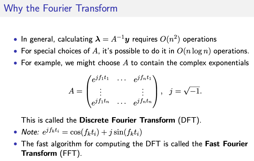
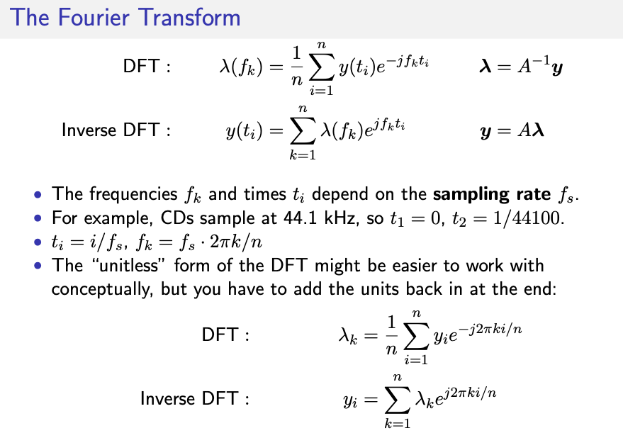
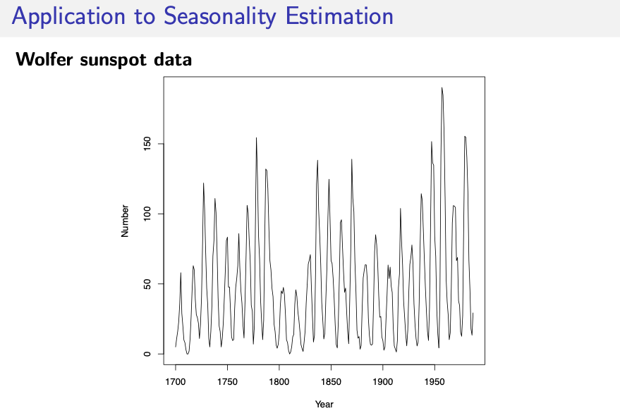
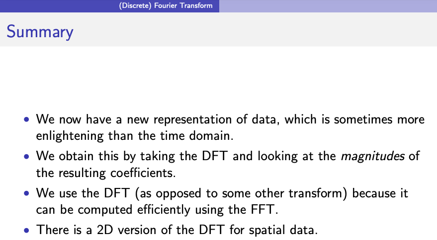
(Discrete) Fourier Transform

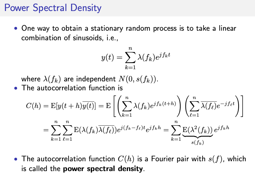
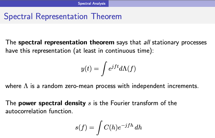
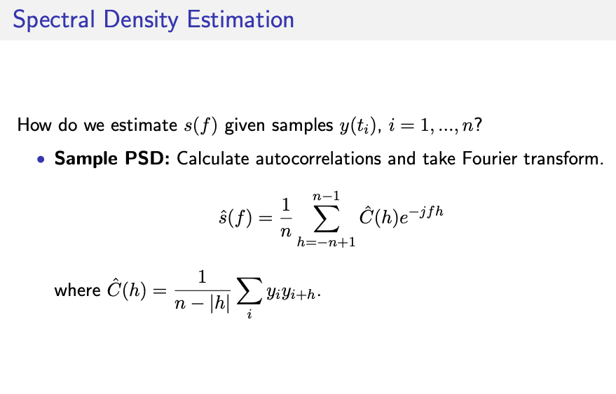
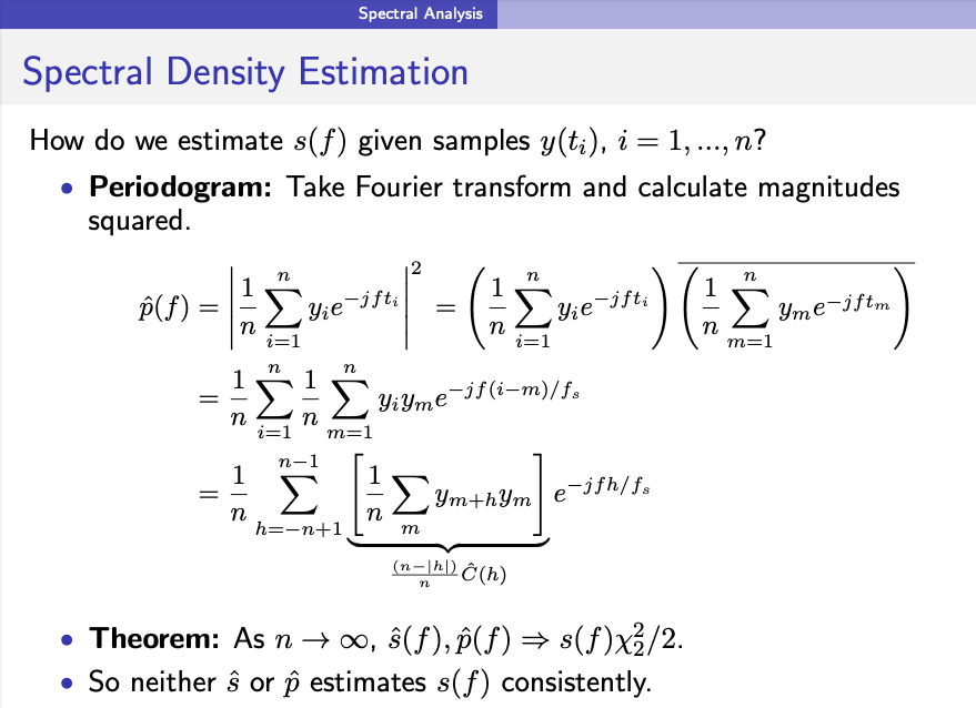
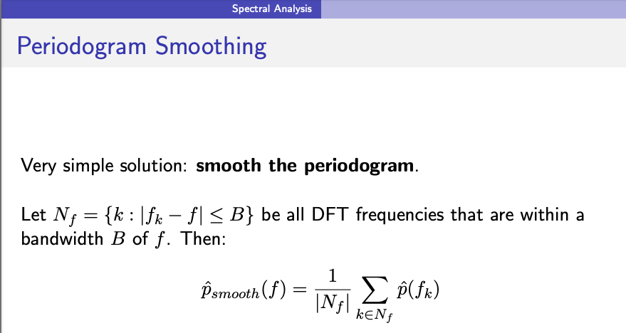
Spectral Analysis

This is a new course.

• The material that we will be covering has not really been synthesized—because it is at the frontiers of statistics!

• We will be loosely following the books

• Shumway and Stoffer. Time Series Analysis and Applications (with R

Applications).

• Sherman. Spatial Statistics and Spatio-Temporal Data.

• You don’t have to purchase these books: they are available for free for Stanford students. (Link on course website.)

• Other useful references:

• Bivand et al. Applied Spatial Data Analysis with R. (also available free) • Cressie and Wikle. Statistics for Spatio-Temporal Data.

点击查看代码