使用sklearn和caffe进行逻辑回归 | Brewing Logistic Regression then Going Deeper
原文首发于个人博客https://kezunlin.me/post/c50b0018/,欢迎阅读!
Brewing Logistic Regression then Going Deeper.
Brewing Logistic Regression then Going Deeper
While Caffe is made for deep networks it can likewise represent "shallow" models like logistic regression for classification. We'll do simple logistic regression on synthetic data that we'll generate and save to HDF5 to feed vectors to Caffe. Once that model is done, we'll add layers to improve accuracy. That's what Caffe is about: define a model, experiment, and then deploy.
import numpy as np

import matplotlib.pyplot as plt

%matplotlib inline

import os

os.chdir('..')

import sys

sys.path.insert(0, './python')

import caffe

import os

import h5py

import shutil

import tempfile

import sklearn

import sklearn.datasets

import sklearn.linear_model

import pandas as pd
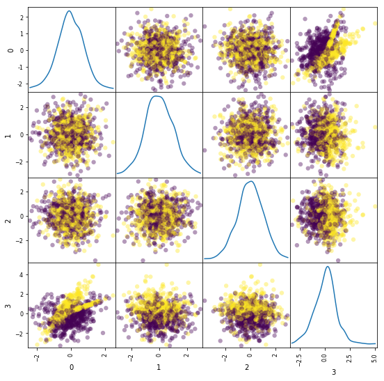
Synthesize a dataset of 10,000 4-vectors for binary classification with 2 informative features and 2 noise features.
X, y = sklearn.datasets.make_classification(

    n_samples=10000, n_features=4, n_redundant=0, n_informative=2,

    n_clusters_per_class=2, hypercube=False, random_state=0

)

print 'data,',X.shape,y.shape # (10000, 4) (10000,) x0,x1,x2,x3, y

# Split into train and test

X, Xt, y, yt = sklearn.model_selection.train_test_split(X, y)

print 'train,',X.shape,y.shape  #train: (7500, 4) (7500,)

print 'test,', Xt.shape,yt.shape#test:  (2500, 4) (2500,)

# Visualize sample of the data

ind = np.random.permutation(X.shape[0])[:1000] # (7500,)--->(1000,)   x0,x1,x2,x3, y

df = pd.DataFrame(X[ind])

_ = pd.plotting.scatter_matrix(df, figsize=(9, 9), diagonal='kde', marker='o', s=40, alpha=.4, c=y[ind])
data, (10000, 4) (10000,)

train, (7500, 4) (7500,)

test, (2500, 4) (2500,)
Learn and evaluate scikit-learn's logistic regression with stochastic gradient descent (SGD) training. Time and check the classifier's accuracy.
%%timeit

# Train and test the scikit-learn SGD logistic regression.

clf = sklearn.linear_model.SGDClassifier(

    loss='log', n_iter=1000, penalty='l2', alpha=5e-4, class_weight='balanced')

clf.fit(X, y)

yt_pred = clf.predict(Xt)

print('Accuracy: {:.3f}'.format(sklearn.metrics.accuracy_score(yt, yt_pred)))
Accuracy: 0.781

Accuracy: 0.781

Accuracy: 0.781

Accuracy: 0.781

1 loop, best of 3: 372 ms per loop
Save the dataset to HDF5 for loading in Caffe.
# Write out the data to HDF5 files in a temp directory.

# This file is assumed to be caffe_root/examples/hdf5_classification.ipynb

dirname = os.path.abspath('./examples/hdf5_classification/data')

if not os.path.exists(dirname):

    os.makedirs(dirname)

train_filename = os.path.join(dirname, 'train.h5')

test_filename = os.path.join(dirname, 'test.h5')

# HDF5DataLayer source should be a file containing a list of HDF5 filenames.

# To show this off, we'll list the same data file twice.

with h5py.File(train_filename, 'w') as f:

    f['data'] = X

    f['label'] = y.astype(np.float32)

with open(os.path.join(dirname, 'train.txt'), 'w') as f:

    f.write(train_filename + '\n')

    f.write(train_filename + '\n')

# HDF5 is pretty efficient, but can be further compressed.

comp_kwargs = {'compression': 'gzip', 'compression_opts': 1}

with h5py.File(test_filename, 'w') as f:

    f.create_dataset('data', data=Xt, **comp_kwargs)

    f.create_dataset('label', data=yt.astype(np.float32), **comp_kwargs)

with open(os.path.join(dirname, 'test.txt'), 'w') as f:

    f.write(test_filename + '\n')
Let's define logistic regression in Caffe through Python net specification. This is a quick and natural way to define nets that sidesteps manually editing the protobuf model.
from caffe import layers as L

from caffe import params as P

def logreg(hdf5, batch_size):

    # logistic regression: data, matrix multiplication, and 2-class softmax loss

    n = caffe.NetSpec()

    n.data, n.label = L.HDF5Data(batch_size=batch_size, source=hdf5, ntop=2)

    n.ip1 = L.InnerProduct(n.data, num_output=2, weight_filler=dict(type='xavier'))

    n.accuracy = L.Accuracy(n.ip1, n.label)

    n.loss = L.SoftmaxWithLoss(n.ip1, n.label)

    return n.to_proto()

train_net_path = 'examples/hdf5_classification/logreg_auto_train.prototxt'

with open(train_net_path, 'w') as f:

    f.write(str(logreg('examples/hdf5_classification/data/train.txt', 10)))

test_net_path = 'examples/hdf5_classification/logreg_auto_test.prototxt'

with open(test_net_path, 'w') as f:

    f.write(str(logreg('examples/hdf5_classification/data/test.txt', 10)))
Now, we'll define our "solver" which trains the network by specifying the locations of the train and test nets we defined above, as well as setting values for various parameters used for learning, display, and "snapshotting".
from caffe.proto import caffe_pb2

def solver(train_net_path, test_net_path):

    s = caffe_pb2.SolverParameter()

    # Specify locations of the train and test networks.

    s.train_net = train_net_path

    s.test_net.append(test_net_path)

    s.test_interval = 1000  # Test after every 1000 training iterations.

    s.test_iter.append(250) # Test 250 "batches" each time we test.

    s.max_iter = 10000      # # of times to update the net (training iterations)

    # Set the initial learning rate for stochastic gradient descent (SGD).

    s.base_lr = 0.01

    # Set `lr_policy` to define how the learning rate changes during training.

    # Here, we 'step' the learning rate by multiplying it by a factor `gamma`

    # every `stepsize` iterations.

    s.lr_policy = 'step'

    s.gamma = 0.1

    s.stepsize = 5000

    # Set other optimization parameters. Setting a non-zero `momentum` takes a

    # weighted average of the current gradient and previous gradients to make

    # learning more stable. L2 weight decay regularizes learning, to help prevent

    # the model from overfitting.

    s.momentum = 0.9

    s.weight_decay = 5e-4

    # Display the current training loss and accuracy every 1000 iterations.

    s.display = 1000

    # Snapshots are files used to store networks we've trained.  Here, we'll

    # snapshot every 10K iterations -- just once at the end of training.

    # For larger networks that take longer to train, you may want to set

    # snapshot < max_iter to save the network and training state to disk during

    # optimization, preventing disaster in case of machine crashes, etc.

    s.snapshot = 10000

    s.snapshot_prefix = 'examples/hdf5_classification/data/train'

    # We'll train on the CPU for fair benchmarking against scikit-learn.

    # Changing to GPU should result in much faster training!

    s.solver_mode = caffe_pb2.SolverParameter.CPU

    return s

solver_path = 'examples/hdf5_classification/logreg_solver.prototxt'

with open(solver_path, 'w') as f:

    f.write(str(solver(train_net_path, test_net_path)))
Time to learn and evaluate our Caffeinated logistic regression in Python.
%%timeit

caffe.set_mode_cpu()

solver = caffe.get_solver(solver_path)

solver.solve()

accuracy = 0

batch_size = solver.test_nets[0].blobs['data'].num

test_iters = int(len(Xt) / batch_size)

for i in range(test_iters):

    solver.test_nets[0].forward()

    accuracy += solver.test_nets[0].blobs['accuracy'].data

accuracy /= test_iters

print("Accuracy: {:.3f}".format(accuracy))
Accuracy: 0.770

Accuracy: 0.770

Accuracy: 0.770

Accuracy: 0.770

1 loop, best of 3: 195 ms per loop
Do the same through the command line interface for detailed output on the model and solving.
!./build/tools/caffe train -solver examples/hdf5_classification/logreg_solver.prototxt
I0224 00:32:03.232779   655 caffe.cpp:178] Use CPU.

I0224 00:32:03.391911   655 solver.cpp:48] Initializing solver from parameters:

train_net: "examples/hdf5_classification/logreg_auto_train.prototxt"

test_net: "examples/hdf5_classification/logreg_auto_test.prototxt"

......

I0224 00:32:04.087514   655 solver.cpp:406]     Test net output #0: accuracy = 0.77

I0224 00:32:04.087532   655 solver.cpp:406]     Test net output #1: loss = 0.593815 (* 1 = 0.593815 loss)

I0224 00:32:04.087541   655 solver.cpp:323] Optimization Done.

I0224 00:32:04.087548   655 caffe.cpp:222] Optimization Done.
If you look at output or the logreg_auto_train.prototxt, you'll see that the model is simple logistic regression.
We can make it a little more advanced by introducing a non-linearity between weights that take the input and weights that give the output -- now we have a two-layer network.
That network is given in nonlinear_auto_train.prototxt, and that's the only change made in nonlinear_logreg_solver.prototxt which we will now use.
The final accuracy of the new network should be higher than logistic regression!
from caffe import layers as L

from caffe import params as P

def nonlinear_net(hdf5, batch_size):

    # one small nonlinearity, one leap for model kind

    n = caffe.NetSpec()

    n.data, n.label = L.HDF5Data(batch_size=batch_size, source=hdf5, ntop=2)

    # define a hidden layer of dimension 40

    n.ip1 = L.InnerProduct(n.data, num_output=40, weight_filler=dict(type='xavier'))

    # transform the output through the ReLU (rectified linear) non-linearity

    n.relu1 = L.ReLU(n.ip1, in_place=True)

    # score the (now non-linear) features

    n.ip2 = L.InnerProduct(n.ip1, num_output=2, weight_filler=dict(type='xavier'))

    # same accuracy and loss as before

    n.accuracy = L.Accuracy(n.ip2, n.label)

    n.loss = L.SoftmaxWithLoss(n.ip2, n.label)

    return n.to_proto()

train_net_path = 'examples/hdf5_classification/nonlinear_auto_train.prototxt'

with open(train_net_path, 'w') as f:

    f.write(str(nonlinear_net('examples/hdf5_classification/data/train.txt', 10)))

test_net_path = 'examples/hdf5_classification/nonlinear_auto_test.prototxt'

with open(test_net_path, 'w') as f:

    f.write(str(nonlinear_net('examples/hdf5_classification/data/test.txt', 10)))

solver_path = 'examples/hdf5_classification/nonlinear_logreg_solver.prototxt'

with open(solver_path, 'w') as f:

    f.write(str(solver(train_net_path, test_net_path)))
%%timeit

caffe.set_mode_cpu()

solver = caffe.get_solver(solver_path)

solver.solve()

accuracy = 0

batch_size = solver.test_nets[0].blobs['data'].num

test_iters = int(len(Xt) / batch_size)

for i in range(test_iters):

    solver.test_nets[0].forward()

    accuracy += solver.test_nets[0].blobs['accuracy'].data

accuracy /= test_iters

print("Accuracy: {:.3f}".format(accuracy))
Accuracy: 0.838

Accuracy: 0.837

Accuracy: 0.838

Accuracy: 0.834

1 loop, best of 3: 277 ms per loop
Do the same through the command line interface for detailed output on the model and solving.
!./build/tools/caffe train -solver examples/hdf5_classification/nonlinear_logreg_solver.prototxt
I0224 00:32:05.654265   658 caffe.cpp:178] Use CPU.

I0224 00:32:05.810444   658 solver.cpp:48] Initializing solver from parameters:

train_net: "examples/hdf5_classification/nonlinear_auto_train.prototxt"

test_net: "examples/hdf5_classification/nonlinear_auto_test.prototxt"

......

I0224 00:32:06.078208   658 solver.cpp:406]     Test net output #0: accuracy = 0.8388

I0224 00:32:06.078225   658 solver.cpp:406]     Test net output #1: loss = 0.382042 (* 1 = 0.382042 loss)

I0224 00:32:06.078234   658 solver.cpp:323] Optimization Done.

I0224 00:32:06.078241   658 caffe.cpp:222] Optimization Done.
# Clean up (comment this out if you want to examine the hdf5_classification/data directory).

shutil.rmtree(dirname)
Reference
History
- 20180102: created.
Copyright
- Post author: kezunlin
- Post link: https://kezunlin.me/post/c50b0018/
- Copyright Notice: All articles in this blog are licensed under CC BY-NC-SA 3.0 unless stating additionally.
Brewing Logistic Regression then Going Deeper.
Brewing Logistic Regression then Going Deeper
While Caffe is made for deep networks it can likewise represent "shallow" models like logistic regression for classification. We'll do simple logistic regression on synthetic data that we'll generate and save to HDF5 to feed vectors to Caffe. Once that model is done, we'll add layers to improve accuracy. That's what Caffe is about: define a model, experiment, and then deploy.
import numpy as np

import matplotlib.pyplot as plt

%matplotlib inline

import os

os.chdir('..')

import sys

sys.path.insert(0, './python')

import caffe

import os

import h5py

import shutil

import tempfile

import sklearn

import sklearn.datasets

import sklearn.linear_model

import pandas as pd
Synthesize a dataset of 10,000 4-vectors for binary classification with 2 informative features and 2 noise features.
X, y = sklearn.datasets.make_classification(

    n_samples=10000, n_features=4, n_redundant=0, n_informative=2,

    n_clusters_per_class=2, hypercube=False, random_state=0

)

print 'data,',X.shape,y.shape # (10000, 4) (10000,) x0,x1,x2,x3, y

# Split into train and test

X, Xt, y, yt = sklearn.model_selection.train_test_split(X, y)

print 'train,',X.shape,y.shape  #train: (7500, 4) (7500,)

print 'test,', Xt.shape,yt.shape#test:  (2500, 4) (2500,)

# Visualize sample of the data

ind = np.random.permutation(X.shape[0])[:1000] # (7500,)--->(1000,)   x0,x1,x2,x3, y

df = pd.DataFrame(X[ind])

_ = pd.plotting.scatter_matrix(df, figsize=(9, 9), diagonal='kde', marker='o', s=40, alpha=.4, c=y[ind])
data, (10000, 4) (10000,)

train, (7500, 4) (7500,)

test, (2500, 4) (2500,)

Learn and evaluate scikit-learn's logistic regression with stochastic gradient descent (SGD) training. Time and check the classifier's accuracy.
%%timeit

# Train and test the scikit-learn SGD logistic regression.

clf = sklearn.linear_model.SGDClassifier(

    loss='log', n_iter=1000, penalty='l2', alpha=5e-4, class_weight='balanced')

clf.fit(X, y)

yt_pred = clf.predict(Xt)

print('Accuracy: {:.3f}'.format(sklearn.metrics.accuracy_score(yt, yt_pred)))
Accuracy: 0.781

Accuracy: 0.781

Accuracy: 0.781

Accuracy: 0.781

1 loop, best of 3: 372 ms per loop
Save the dataset to HDF5 for loading in Caffe.
# Write out the data to HDF5 files in a temp directory.

# This file is assumed to be caffe_root/examples/hdf5_classification.ipynb

dirname = os.path.abspath('./examples/hdf5_classification/data')

if not os.path.exists(dirname):

    os.makedirs(dirname)

train_filename = os.path.join(dirname, 'train.h5')

test_filename = os.path.join(dirname, 'test.h5')

# HDF5DataLayer source should be a file containing a list of HDF5 filenames.

# To show this off, we'll list the same data file twice.

with h5py.File(train_filename, 'w') as f:

    f['data'] = X

    f['label'] = y.astype(np.float32)

with open(os.path.join(dirname, 'train.txt'), 'w') as f:

    f.write(train_filename + '\n')

    f.write(train_filename + '\n')

# HDF5 is pretty efficient, but can be further compressed.

comp_kwargs = {'compression': 'gzip', 'compression_opts': 1}

with h5py.File(test_filename, 'w') as f:

    f.create_dataset('data', data=Xt, **comp_kwargs)

    f.create_dataset('label', data=yt.astype(np.float32), **comp_kwargs)

with open(os.path.join(dirname, 'test.txt'), 'w') as f:

    f.write(test_filename + '\n')
Let's define logistic regression in Caffe through Python net specification. This is a quick and natural way to define nets that sidesteps manually editing the protobuf model.
from caffe import layers as L

from caffe import params as P

def logreg(hdf5, batch_size):

    # logistic regression: data, matrix multiplication, and 2-class softmax loss

    n = caffe.NetSpec()

    n.data, n.label = L.HDF5Data(batch_size=batch_size, source=hdf5, ntop=2)

    n.ip1 = L.InnerProduct(n.data, num_output=2, weight_filler=dict(type='xavier'))

    n.accuracy = L.Accuracy(n.ip1, n.label)

    n.loss = L.SoftmaxWithLoss(n.ip1, n.label)

    return n.to_proto()

train_net_path = 'examples/hdf5_classification/logreg_auto_train.prototxt'

with open(train_net_path, 'w') as f:

    f.write(str(logreg('examples/hdf5_classification/data/train.txt', 10)))

test_net_path = 'examples/hdf5_classification/logreg_auto_test.prototxt'

with open(test_net_path, 'w') as f:

    f.write(str(logreg('examples/hdf5_classification/data/test.txt', 10)))
Now, we'll define our "solver" which trains the network by specifying the locations of the train and test nets we defined above, as well as setting values for various parameters used for learning, display, and "snapshotting".
from caffe.proto import caffe_pb2

def solver(train_net_path, test_net_path):

    s = caffe_pb2.SolverParameter()

    # Specify locations of the train and test networks.

    s.train_net = train_net_path

    s.test_net.append(test_net_path)

    s.test_interval = 1000  # Test after every 1000 training iterations.

    s.test_iter.append(250) # Test 250 "batches" each time we test.

    s.max_iter = 10000      # # of times to update the net (training iterations)

    # Set the initial learning rate for stochastic gradient descent (SGD).

    s.base_lr = 0.01

    # Set `lr_policy` to define how the learning rate changes during training.

    # Here, we 'step' the learning rate by multiplying it by a factor `gamma`

    # every `stepsize` iterations.

    s.lr_policy = 'step'

    s.gamma = 0.1

    s.stepsize = 5000

    # Set other optimization parameters. Setting a non-zero `momentum` takes a

    # weighted average of the current gradient and previous gradients to make

    # learning more stable. L2 weight decay regularizes learning, to help prevent

    # the model from overfitting.

    s.momentum = 0.9

    s.weight_decay = 5e-4

    # Display the current training loss and accuracy every 1000 iterations.

    s.display = 1000

    # Snapshots are files used to store networks we've trained.  Here, we'll

    # snapshot every 10K iterations -- just once at the end of training.

    # For larger networks that take longer to train, you may want to set

    # snapshot < max_iter to save the network and training state to disk during

    # optimization, preventing disaster in case of machine crashes, etc.

    s.snapshot = 10000

    s.snapshot_prefix = 'examples/hdf5_classification/data/train'

    # We'll train on the CPU for fair benchmarking against scikit-learn.

    # Changing to GPU should result in much faster training!

    s.solver_mode = caffe_pb2.SolverParameter.CPU

    return s

solver_path = 'examples/hdf5_classification/logreg_solver.prototxt'

with open(solver_path, 'w') as f:

    f.write(str(solver(train_net_path, test_net_path)))
Time to learn and evaluate our Caffeinated logistic regression in Python.
%%timeit

caffe.set_mode_cpu()

solver = caffe.get_solver(solver_path)

solver.solve()

accuracy = 0

batch_size = solver.test_nets[0].blobs['data'].num

test_iters = int(len(Xt) / batch_size)

for i in range(test_iters):

    solver.test_nets[0].forward()

    accuracy += solver.test_nets[0].blobs['accuracy'].data

accuracy /= test_iters

print("Accuracy: {:.3f}".format(accuracy))
Accuracy: 0.770

Accuracy: 0.770

Accuracy: 0.770

Accuracy: 0.770

1 loop, best of 3: 195 ms per loop
Do the same through the command line interface for detailed output on the model and solving.
!./build/tools/caffe train -solver examples/hdf5_classification/logreg_solver.prototxt
I0224 00:32:03.232779   655 caffe.cpp:178] Use CPU.

I0224 00:32:03.391911   655 solver.cpp:48] Initializing solver from parameters:

train_net: "examples/hdf5_classification/logreg_auto_train.prototxt"

test_net: "examples/hdf5_classification/logreg_auto_test.prototxt"

......

I0224 00:32:04.087514   655 solver.cpp:406]     Test net output #0: accuracy = 0.77

I0224 00:32:04.087532   655 solver.cpp:406]     Test net output #1: loss = 0.593815 (* 1 = 0.593815 loss)

I0224 00:32:04.087541   655 solver.cpp:323] Optimization Done.

I0224 00:32:04.087548   655 caffe.cpp:222] Optimization Done.
If you look at output or the logreg_auto_train.prototxt, you'll see that the model is simple logistic regression.
We can make it a little more advanced by introducing a non-linearity between weights that take the input and weights that give the output -- now we have a two-layer network.
That network is given in nonlinear_auto_train.prototxt, and that's the only change made in nonlinear_logreg_solver.prototxt which we will now use.
The final accuracy of the new network should be higher than logistic regression!
from caffe import layers as L

from caffe import params as P

def nonlinear_net(hdf5, batch_size):

    # one small nonlinearity, one leap for model kind

    n = caffe.NetSpec()

    n.data, n.label = L.HDF5Data(batch_size=batch_size, source=hdf5, ntop=2)

    # define a hidden layer of dimension 40

    n.ip1 = L.InnerProduct(n.data, num_output=40, weight_filler=dict(type='xavier'))

    # transform the output through the ReLU (rectified linear) non-linearity

    n.relu1 = L.ReLU(n.ip1, in_place=True)

    # score the (now non-linear) features

    n.ip2 = L.InnerProduct(n.ip1, num_output=2, weight_filler=dict(type='xavier'))

    # same accuracy and loss as before

    n.accuracy = L.Accuracy(n.ip2, n.label)

    n.loss = L.SoftmaxWithLoss(n.ip2, n.label)

    return n.to_proto()

train_net_path = 'examples/hdf5_classification/nonlinear_auto_train.prototxt'

with open(train_net_path, 'w') as f:

    f.write(str(nonlinear_net('examples/hdf5_classification/data/train.txt', 10)))

test_net_path = 'examples/hdf5_classification/nonlinear_auto_test.prototxt'

with open(test_net_path, 'w') as f:

    f.write(str(nonlinear_net('examples/hdf5_classification/data/test.txt', 10)))

solver_path = 'examples/hdf5_classification/nonlinear_logreg_solver.prototxt'

with open(solver_path, 'w') as f:

    f.write(str(solver(train_net_path, test_net_path)))
%%timeit

caffe.set_mode_cpu()

solver = caffe.get_solver(solver_path)

solver.solve()

accuracy = 0

batch_size = solver.test_nets[0].blobs['data'].num

test_iters = int(len(Xt) / batch_size)

for i in range(test_iters):

    solver.test_nets[0].forward()

    accuracy += solver.test_nets[0].blobs['accuracy'].data

accuracy /= test_iters

print("Accuracy: {:.3f}".format(accuracy))
Accuracy: 0.838

Accuracy: 0.837

Accuracy: 0.838

Accuracy: 0.834

1 loop, best of 3: 277 ms per loop
Do the same through the command line interface for detailed output on the model and solving.
!./build/tools/caffe train -solver examples/hdf5_classification/nonlinear_logreg_solver.prototxt
I0224 00:32:05.654265   658 caffe.cpp:178] Use CPU.

I0224 00:32:05.810444   658 solver.cpp:48] Initializing solver from parameters:

train_net: "examples/hdf5_classification/nonlinear_auto_train.prototxt"

test_net: "examples/hdf5_classification/nonlinear_auto_test.prototxt"

......

I0224 00:32:06.078208   658 solver.cpp:406]     Test net output #0: accuracy = 0.8388

I0224 00:32:06.078225   658 solver.cpp:406]     Test net output #1: loss = 0.382042 (* 1 = 0.382042 loss)

I0224 00:32:06.078234   658 solver.cpp:323] Optimization Done.

I0224 00:32:06.078241   658 caffe.cpp:222] Optimization Done.
# Clean up (comment this out if you want to examine the hdf5_classification/data directory).

shutil.rmtree(dirname)
Reference
History
- 20180102: created.
Copyright
- Post author: kezunlin
- Post link: https://kezunlin.me/post/c50b0018/
- Copyright Notice: All articles in this blog are licensed under CC BY-NC-SA 3.0 unless stating additionally.
使用sklearn和caffe进行逻辑回归 | Brewing Logistic Regression then Going Deeper的更多相关文章
- 通俗地说逻辑回归【Logistic regression】算法(二)sklearn逻辑回归实战
前情提要: 通俗地说逻辑回归[Logistic regression]算法(一) 逻辑回归模型原理介绍 上一篇主要介绍了逻辑回归中,相对理论化的知识,这次主要是对上篇做一点点补充,以及介绍sklear ...
- 逻辑回归(Logistic Regression)算法小结
一.逻辑回归简述: 回顾线性回归算法,对于给定的一些n维特征(x1,x2,x3,......xn),我们想通过对这些特征进行加权求和汇总的方法来描绘出事物的最终运算结果.从而衍生出我们线性回归的计算公 ...
- 机器学习二 逻辑回归作业、逻辑回归(Logistic Regression)
机器学习二 逻辑回归作业 作业在这,http://speech.ee.ntu.edu.tw/~tlkagk/courses/ML_2016/Lecture/hw2.pdf 是区分spam的. 57 ...
- Python实践之(七)逻辑回归(Logistic Regression)
机器学习算法与Python实践之(七)逻辑回归(Logistic Regression) zouxy09@qq.com http://blog.csdn.net/zouxy09 机器学习算法与Pyth ...
- 逻辑回归模型(Logistic Regression, LR)基础
逻辑回归模型(Logistic Regression, LR)基础 逻辑回归(Logistic Regression, LR)模型其实仅在线性回归的基础上,套用了一个逻辑函数,但也就由于这个逻辑函 ...
- 机器学习算法与Python实践之(七)逻辑回归(Logistic Regression)
http://blog.csdn.net/zouxy09/article/details/20319673 机器学习算法与Python实践之(七)逻辑回归(Logistic Regression) z ...
- 机器学习/逻辑回归(logistic regression)/--附python代码
个人分类: 机器学习 本文为吴恩达<机器学习>课程的读书笔记,并用python实现. 前一篇讲了线性回归,这一篇讲逻辑回归,有了上一篇的基础,这一篇的内容会显得比较简单. 逻辑回归(log ...
- Python机器学习算法 — 逻辑回归(Logistic Regression)
逻辑回归--简介 逻辑回归(Logistic Regression)就是这样的一个过程:面对一个回归或者分类问题,建立代价函数,然后通过优化方法迭代求解出最优的模型参数,然后测试验证我们这个求解的模型 ...
- [机器学习] Coursera ML笔记 - 逻辑回归(Logistic Regression)
引言 机器学习栏目记录我在学习Machine Learning过程的一些心得笔记,涵盖线性回归.逻辑回归.Softmax回归.神经网络和SVM等等.主要学习资料来自Standford Andrew N ...
随机推荐
- HTML5+WebGL 的加油站 3D 可视化监控
前言 随着数字化,工业互联网,物联网的发展,我国加油站正向有人值守,无人操作,远程控制的方向发展,传统的人工巡查方式逐渐转变为以自动化控制为主的在线监控方式,即采用数据采集与监控系统 SCADA.SC ...
- 基于docker的mysql8的主从复制
基于docker的mysql8的主从复制 创建mysql的docker镜像 构建docker镜像,其中数据卷配置内容在下面,结构目录如下 version: '3.7' services: db: # ...
- python3.x以上 爬虫 使用问题 urllib(不能使用urllib2)
问题一: python 3.x 以上版本揽括了 urllib2,把urllib2 和 urllib 整合到一起. 并且引入模块变成一个,只有 import urllib # import urllib ...
- solr学习篇(三) solr7.4 连接MySQL数据库
目录 导入相关jar包 配置连接信息 将数据库导入到solr中 验证是否成功 创建一个Core,创建Core的方法之前已经很详细的讲解过了,如果还是不清楚请参考 solr7.4 安装配置篇: 1.导入 ...
- GO基础之闭包
一.闭包的理解 闭包是匿名函数与匿名函数所引用环境的组合.匿名函数有动态创建的特性,该特性使得匿名函数不用通过参数传递的方式,就可以直接引用外部的变量. 这就类似于常规函数直接使用全局变量一样,个人理 ...
- fenby C语言 P16
while先判断,不符合,不执行 dowhile后判断,不符合,执行一次 #include <stdio.h> int main(){ int i=1,sum=0; do{ sum=sum ...
- SpringCloud之Nacos服务注册(十八)
一 服务提供配置 pom.xml <dependency> <groupId>org.springframework.boot</groupId> <arti ...
- 【网络安全】HTTPS为什么比较安全
目录 HTTP和HTTPS简介 SSL协议 SSL协议的主要功能 SSL协议加密数据的原理 用户和服务器的认证流程 TLS 参考 HTTP和HTTPS简介 1. HTTP协议为什么是不安全的 http ...
- quartus使用串口IP模块
在quartus平台中使用串口模块的IP,需要使用到platform designer软件来实现. 1.在quartus界面调出IP Catalog界面. 2.在IP catalog中搜索UART,找 ...
- [Next] Next.js+Nest.js实现GitHub第三方登录
GitHub OAuth 第三方登录 第三方登录的关键知识点就是 OAuth2.0 . 第三方登录,实质就是 OAuth 授权 . OAuth 是一个开放标准,允许用户让第三方应用访问某一个网站的资源 ...