python3 networkx

一.networkx

1.用于图论和复杂网络

2.官网：http://networkx.github.io/

3.networkx常常结合numpy等数据处理相关的库一起使用，通过matplot来可视化图

二.绘制图

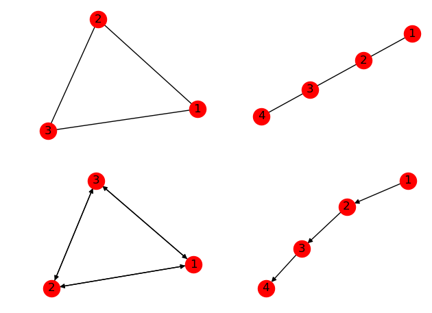
1.创建图

 import networkx as nx
 import matplotlib.pyplot as plt

 G=nx.Graph()#创建空图，无向图
 # G1=nx.DiGraph(e)#创建空图，有向图
 # G = nx.Graph(name='my graph')#指定图的属性（name） 的值（my graph）
 G.add_edges_from(([1,2],[2,3],[3,1]))

 e = [(1, 2), (2, 3), (3, 4)]  # 边的列表
 G2 = nx.Graph(e)#根据e来创建图

 F=G.to_directed()#把无向图转换为有向图

 #创建多图，类MultiGraph和类MultiDiGraph允许添加相同的边两次，这两条边可能附带不同的权值
 # H=nx.MultiGraph(e)
 H=nx.MultiDiGraph(e)

 plt.subplot(2,2,1)
 nx.draw(G,with_labels=True)
 plt.subplot(2,2,2)
 nx.draw(G2,with_labels=True)
 plt.subplot(2,2,3)
 nx.draw(F,with_labels=True)
 plt.subplot(2,2,4)
 nx.draw(H,with_labels=True)

 plt.show()

创建图

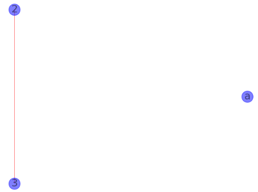
2.无向图

 import networkx as nx
 import matplotlib.pyplot as plt

 G=nx.Graph()#创建空图

 #添加节点
 G.add_node('a')
 G.add_node(1)                  #添加单个节点
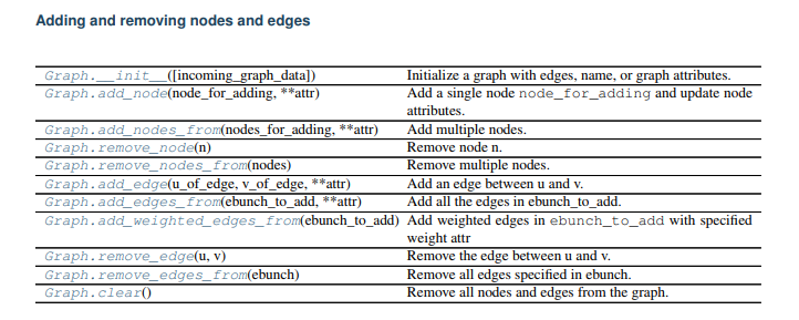
 G.add_nodes_from([2,3,4])      #添加一些节点，容器，（可以是list, dict, set，）

 #添加边，如果点不在图中，会自动创建点
 G.add_edge(1,'a',weight=1.2)   #添加单条边，连接1，‘a’的边,可以赋予边属性以及他的值
 G.add_edges_from([(2,3),(3,4)])#添加一些边（列表）
 G.add_weighted_edges_from([(1,'a',0.1),(4,2,0.5)])#给边赋予权重

 #移除边
 G.remove_edge(2,4)             #移除一条边
 G.remove_edges_from([(3,4),])  #移除一些边

 #移除节点,同时移除他对应的边
 G.remove_node(1)               #移除单个节点
 G.remove_nodes_from([4,])      #移除一些节点

 #绘图
 nx.draw(G,                          # 图
         pos=nx.circular_layout(G),  # 图的布局
         alpha=0.5,                  # 图的透明度（默认1.0不透明，0完全透明）

         with_labels=True,           # 节点是否带标签
         font_size=18,               # 节点标签字体大小
         node_size=400,              # 指定节点的尺寸大小
         node_color='blue',          # 指定节点的颜色
         node_shape='o',             # 节点的形状

         edge_color='r',             # 边的颜色
         width=0.8,                  # 边的宽度
         style='solid',              # 边的样式

         ax=None,                    # Matplotlib Axes对象，可选在指定的Matplotlib轴中绘制图形。
         )

 plt.show()

无向图

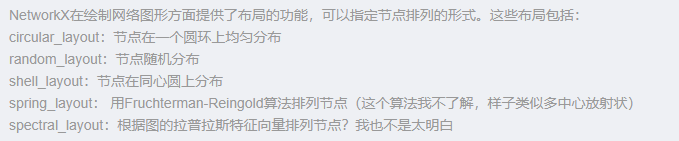
绘图布局

3.有向图和无向图的最大差别在于：有向图中的边是有顺序的，前一个表示开始节点，后一个表示结束节点。

三.图

数据结构

1.图的属性

 #像color,label,weight或者其他Python对象的属性都可以被设置为graph，node，edge的属性
 # 每个graph，node，edge都能够包含key/value这样的字典数据
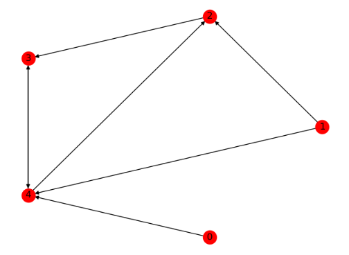
 import networkx as nx
 import matplotlib.pyplot as plt

 G=nx.DiGraph([(1,2),(2,3),(3,4),(1,4),(4,2)],name='my digraph',a='b')
 #创建一个有向图，赋予边，点，权重，以及有向图的属性name的值my digraph

 #属性都可以在定义时赋予,或者通过直接赋值来添加修改
 #图属性
 print(G)#图的名称
 print(G.graph)#图的属性，字典
 G.graph['b']=19#赋予属性
 print(G.graph)
 print('#'*60)

 #节点属性
 print('图的节点：',G.nodes)#列表
 print('节点个数：',G.number_of_nodes())
 G.add_node('b',time='0.2')
 print(G.node['b'])#显示单个节点的信息
 G.node['b']['time']=0.3#修改属性
 print(G.node['b'])
 print('#'*60)

 #边属性
 print('图的边：',G.edges)#列表
 print ('边的个数：',G.number_of_edges())
 G.add_edge('a','b',weight=0.6)
 G.add_edges_from( [ (2,3),(3,4) ], color="red")
 G.add_edges_from( [(1,2,{"color":"blue"}),(4,5,{"weight":8})])
 G[1][2]["width"]=4.7#添加或修改属性
 print(G.get_edge_data(1, 2))#获取某条边的属性
 print('#'*60)

 nx.draw(G,pos = nx.circular_layout(G),with_labels=True)

 plt.show
 --------------------------------------------------------------------------
 my digraph
 {'name': 'my digraph', 'a': 'b'}
 {'name': 'my digraph', 'a': 'b', 'b': 19}
 ############################################################
 图的节点： [1, 2, 3, 4]
 节点个数： 4
 {'time': '0.2'}
 {'time': 0.3}
 {2: {}, 4: {}}
 ############################################################
 图的边： [(1, 2), (1, 4), (2, 3), (3, 4), (4, 2)]
 边的个数： 5
 {'color': 'blue', 'width': 4.7}

属性

2.边和节点

 import networkx as nx
 import matplotlib.pyplot as plt

 G=nx.DiGraph([(1,2,{'weight':10}),(2,3),(3,4),(1,4),(4,2)])

 nx.add_path(G, [0, 4,3])#在图中添加路径

 # 对1节点进行分析
 print(G.node[1])#节点1的信息
 G.node[1]['time']=1#赋予节点属性
 print(G.node[1])
 print(G[1])  # 1相关的节点的信息,他的邻居和对应的边的属性
 print(G.degree(1))  # 1节点的度
 print('#'*60)

 # 对【1】【2】边进行分析
 print(G[1][2])  # 查看某条边的属性
 G[1][2]['weight'] = 0.4  # 重新设置边的权重
 print(G[1][2]['weight'])  # 查看边的权重
 G[1][2]['color'] = 'blue'  # 添加属性
 print(G[1][2])

 nx.draw(G,pos = nx.circular_layout(G),with_labels=True)

 plt.show()
 ------------------------------------------------------------------
 {}
 {'time': 1}
 {2: {'weight': 10}, 4: {}}
 2
 ############################################################
 {'weight': 10}
 0.4
 {'weight': 0.4, 'color': 'blue'}

边和节点

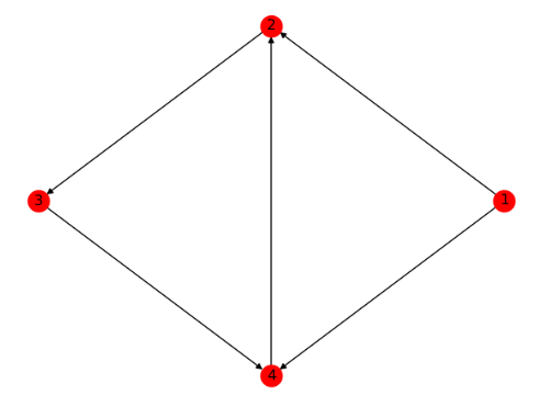
3.有向图

 import networkx as nx
 import matplotlib.pyplot as plt

 G=nx.DiGraph([(1,2,{'weight':10}),(2,3),(3,4),(1,4),(4,2)])
 print('#'*60)
 print(G.edges)#An OutEdgeView of the DiGraph as G.edges or G.edges().
 print(G.out_edges)#An OutEdgeView of the DiGraph as G.edges or G.edges().
 print(G.in_edges)#An InEdgeView of the Graph as G.in_edges or G.in_edges()
 print('#'*60)

 print(G.degree)#图的度
 print(G.out_degree)#图的出度
 print(G.in_degree)#图的入度
 print('#'*60)

 print(G.adj)#Graph adjacency object holding the neighbors of each node
 print(G.neighbors(2))#节点2的邻居
 print(G.succ)#Graph adjacency object holding the successors of each node
 print(G.successors(2))#节点2的后继节点
 print(G.pred)#Graph adjacency object holding the predecessors of each node
 print(G.predecessors(2))#节点2的前继节点
 #以列表形式打印
 print([n for n in G.neighbors(2)])
 print([n for n in G.successors(2)])
 print([n for n in G.predecessors(2)])

 nx.draw(G,pos = nx.circular_layout(G),with_labels=True)

 plt.show()
 --------------------------------------------------------
 ############################################################
 [(1, 2), (1, 4), (2, 3), (3, 4), (4, 2)]
 [(1, 2), (1, 4), (2, 3), (3, 4), (4, 2)]
 [(1, 2), (4, 2), (2, 3), (3, 4), (1, 4)]
 ############################################################
 [(1, 2), (2, 3), (3, 2), (4, 3)]
 [(1, 2), (2, 1), (3, 1), (4, 1)]
 [(1, 0), (2, 2), (3, 1), (4, 2)]
 ############################################################
 {1: {2: {'weight': 10}, 4: {}}, 2: {3: {}}, 3: {4: {}}, 4: {2: {}}}
 <dict_keyiterator object at 0x0DA2BF00>
 {1: {2: {'weight': 10}, 4: {}}, 2: {3: {}}, 3: {4: {}}, 4: {2: {}}}
 <dict_keyiterator object at 0x0DA2BF00>
 {1: {}, 2: {1: {'weight': 10}, 4: {}}, 3: {2: {}}, 4: {3: {}, 1: {}}}
 <dict_keyiterator object at 0x0DA2BF00>
 [3]
 [3]
 [1, 4]

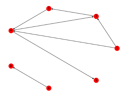
有向图

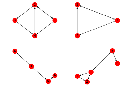
4.图的操作

Applying classic graph operations

 import networkx as nx
 import matplotlib.pyplot as plt

 G=nx.DiGraph([(1,2,{'weight':10}),(2,1,{'weight':1}),(2,3),(3,4),(1,4),(4,2)])
 G2=nx.DiGraph([(1,'a'),('a','b'),(1,4)])

 H=G.subgraph([1,2,4])#产生关于节点的子图

 G3=nx.compose(H,G2)#结合两个图并表示两者共同的节点

 plt.subplot(221)
 nx.draw(G,pos = nx.circular_layout(G),with_labels=True,name='G')

 plt.subplot(222)
 nx.draw(H,pos = nx.circular_layout(G),with_labels=True)

 plt.subplot(223)
 nx.draw(G2,with_labels=True)

 plt.subplot(224)
 nx.draw(G3,with_labels=True)

 plt.show()

生成图

4.算法

...

四.简单根据数据画图

 import networkx as nx
 import matplotlib.pyplot as plt

 #1.导入数据：
 # networkx支持的直接处理的数据文件格式adjlist/edgelist/gexf/gml/pickle/graphml/json/lead/yaml/graph6/sparse6/pajek/shp/
 #根据实际情况，把文件变为gml文件
 G1 = nx.DiGraph()
 with open('file.txt') as f:
     for line in f:
         cell = line.strip().split(',')
         G1.add_weighted_edges_from([(cell[0],cell[1],cell[2])])
     nx.write_gml(G1,'file.gml')#写网络G进GML文件

 G=nx.read_gml("file.gml") #读取gml文件
 # parse_gml(lines[,relael]) 从字符串中解析GML图
 # generate_gml(G)  以gml格式生成一个简单条目的网络G

 print(G.nodes)
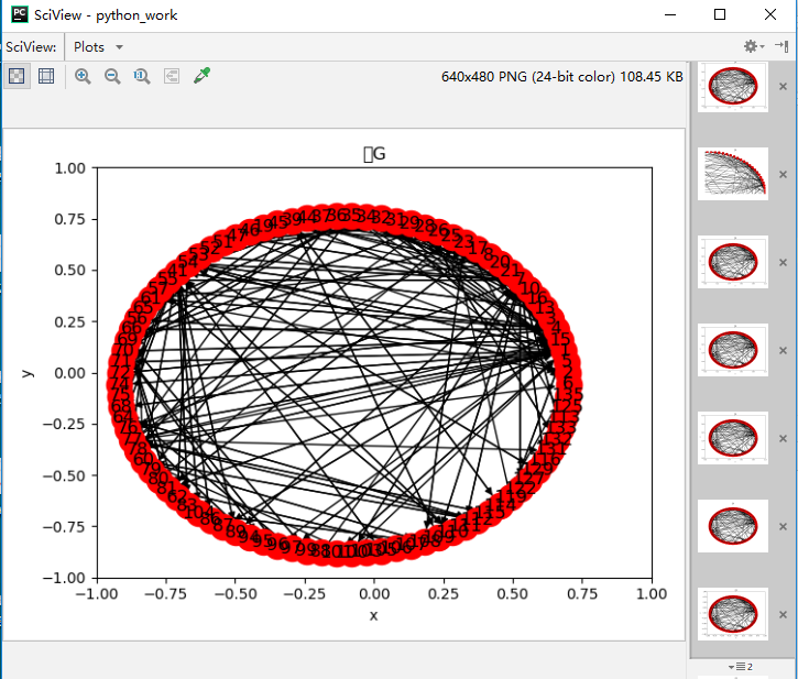
 print(G.edges)

 #2.在figure上先设置坐标
 plt.title("图G")
 plt.ylabel("y")
 plt.xlabel("x")
 plt.xlim(-1,1)
 plt.ylim(-1,1)

 #再在坐标轴里面调节图形大小
 #整个figure按照X与Y轴横竖来平均切分，以0到1之间的数值来表示
 #axes([x,y,xs,ys])，如果不设置
 #其中x代表在X轴的位置，y代表在Y轴的位置，xs代表在X轴上向右延展的范围大小，yx代表在Y轴中向上延展的范围大小
 plt.axes([0.1, 0.1, 0.8, 0.8])

 #3.在axes中绘图
 nx.draw(G,pos = nx.circular_layout(G),with_labels=True,)

 #4.保存图形
 plt.savefig("file.png")#将图像保存到一个文件

 plt.show()
 -----------------------------------------------------
 ['', '', '', '', '', '', '', '', '', '', '', '', '', '', '', '', '', '', '', '', '', '', '', '', '', '', '', '', '', '', '', '', '', '', '', '', '', '', '', '', '', '', '', '', '', '', '', '', '', '', '', '', '', '', '', '', '', '', '', '', '', '', '', '', '', '', '', '', '', '', '', '', '', '', '', '', '', '', '', '', '', '', '', '', '', '', '', '', '', '', '', '', '', '']
 [('', ''), ('', ''), ('', ''), ('', ''), ('', ''), ('', ''), ('', ''), ('', ''), ('', ''), ('', ''), ('', ''), ('', ''), ('', ''), ('', ''), ('', ''), ('', ''), ('', ''), ('', ''), ('', ''), ('', ''), ('', ''), ('', ''), ('', ''), ('', ''), ('', ''), ('', ''), ('', ''), ('', ''), ('', ''), ('', ''), ('', ''), ('', ''), ('', ''), ('', ''), ('', ''), ('', ''), ('', ''), ('', ''), ('', ''), ('', ''), ('', ''), ('', ''), ('', ''), ('', ''), ('', ''), ('', ''), ('', ''), ('', ''), ('', ''), ('', ''), ('', ''), ('', ''), ('', ''), ('', ''), ('', ''), ('', ''), ('', ''), ('', ''), ('', ''), ('', ''), ('', ''), ('', ''), ('', ''), ('', ''), ('', ''), ('', ''), ('', ''), ('', ''), ('', ''), ('', ''), ('', ''), ('', ''), ('', ''), ('', ''), ('', ''), ('', ''), ('', ''), ('', ''), ('', ''), ('', ''), ('', ''), ('', ''), ('', ''), ('', ''), ('', ''), ('', ''), ('', ''), ('', ''), ('', ''), ('', ''), ('', ''), ('', ''), ('', ''), ('', ''), ('', ''), ('', ''), ('', ''), ('', ''), ('', ''), ('', ''), ('', ''), ('', ''), ('', ''), ('', ''), ('', ''), ('', ''), ('', ''), ('', ''), ('', ''), ('', ''), ('', ''), ('', ''), ('', ''), ('', ''), ('', ''), ('', ''), ('', ''), ('', ''), ('', ''), ('', ''), ('', ''), ('', ''), ('', ''), ('', ''), ('', ''), ('', ''), ('', ''), ('', ''), ('', ''), ('', ''), ('', ''), ('', ''), ('', ''), ('', ''), ('', ''), ('', ''), ('', ''), ('', ''), ('', ''), ('', ''), ('', ''), ('', ''), ('', ''), ('', ''), ('', ''), ('', ''), ('', ''), ('', ''), ('', ''), ('', ''), ('', ''), ('', ''), ('', ''), ('', ''), ('', ''), ('', ''), ('', ''), ('', ''), ('', ''), ('', ''), ('', ''), ('', ''), ('', ''), ('', ''), ('', ''), ('', ''), ('', ''), ('', ''), ('', ''), ('', ''), ('', ''), ('', ''), ('', ''), ('', ''), ('', ''), ('', ''), ('', ''), ('', ''), ('', ''), ('', ''), ('', ''), ('', ''), ('', ''), ('', ''), ('', ''), ('', ''), ('', ''), ('', ''), ('', ''), ('', ''), ('', ''), ('', ''), ('', ''), ('', ''), ('', ''), ('', ''), ('', ''), ('', ''), ('', ''), ('', ''), ('', ''), ('', ''), ('', ''), ('', ''), ('', ''), ('', ''), ('', ''), ('', ''), ('', ''), ('', ''), ('', ''), ('', ''), ('', ''), ('', ''), ('', ''), ('', ''), ('', ''), ('', ''), ('', ''), ('', ''), ('', ''), ('', ''), ('', ''), ('', ''), ('', ''), ('', ''), ('', ''), ('', ''), ('', ''), ('', ''), ('', ''), ('', ''), ('', ''), ('', ''), ('', ''), ('', ''), ('', ''), ('', ''), ('', ''), ('', ''), ('', ''), ('', ''), ('', ''), ('', ''), ('', ''), ('', ''), ('', ''), ('', ''), ('', ''), ('', ''), ('', ''), ('', ''), ('', ''), ('', ''), ('', ''), ('', ''), ('', ''), ('', ''), ('', ''), ('', ''), ('', ''), ('', ''), ('', ''), ('', ''), ('', ''), ('', ''), ('', ''), ('', ''), ('', ''), ('', ''), ('', ''), ('', ''), ('', ''), ('', ''), ('', ''), ('', ''), ('', ''), ('', ''), ('', ''), ('', ''), ('', ''), ('', ''), ('', ''), ('', ''), ('', ''), ('', ''), ('', ''), ('', ''), ('', ''), ('', ''), ('', ''), ('', ''), ('', ''), ('', ''), ('', ''), ('', ''), ('', ''), ('', ''), ('', ''), ('', ''), ('', '')]

绘图

5.分析图

 import networkx as nx
 import matplotlib.pyplot as plt

 G=nx.read_gml("file.gml")
 UG=G.to_undirected()

 #网络信息
 print(nx.info(G))
 eccen = nx.eccentricity(UG)#节点离心度
 print(eccen)
 print(max(eccen.values()))
 print(min(eccen.values()))
 # print(nx.diameter(G)) # 网络直径
 # print(nx.radius(G)) #网络半径
 print(nx.average_shortest_path_length(G)) # 网络平均最短距离
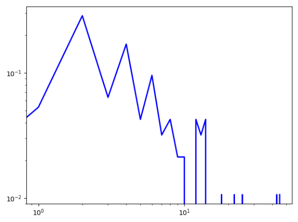
 print(nx.average_shortest_path_length(UG)) # 网络平均最短距离

 #度分布
 degree=nx.degree_histogram(G)#所有节点的度分布序列
 print(degree)
 x=range(len(degree)) #生成x轴序列
 y=[z/float(sum(degree))for z in degree]#将频次转换为频率
 plt.loglog(x,y,color='blue',linewidth=2)#在双对数坐标轴上绘制分布曲线

 #度中心度
 print(nx.degree_centrality(G))#计算每个点的度中心性
 print(nx.in_degree_centrality(G))#计算每个点的入度中心性
 print(nx.out_degree_centrality(G))#计算每个点的出度中心性

 #紧密中心度
 print(nx.closeness_centrality(G))

 #介数中心度
 print(nx.betweenness_centrality(G))

 #特征向量中心度
 print(nx.eigenvector_centrality(G))

 #网络密度
 print(nx.density(G))

 #网络传递性
 print(nx.transitivity(G))

 #网络群聚系数
 print(nx.average_clustering(UG))
 print(nx.clustering(UG))

 #节点度的匹配性
 print(nx.degree_assortativity_coefficient(UG))

 plt.show()
 ------------------------------------------------------------------

分析图

五.补充

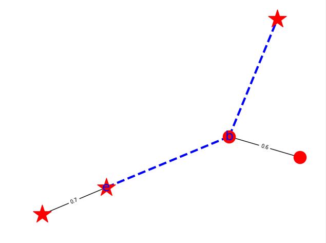
1.更精细地画图，可以绘制特定的边和点，一般默认全画

 import networkx as nx
 import matplotlib.pyplot as plt

 #1.获得带权图
 G = nx.Graph()
 G.add_edges_from([('a', 'b', {'weight':0.6}),
                   ('a', 'c', {'weight':0.2}),
                   ('a', 'd', {'weight':0.1}),
                   ('c', 'e', {'weight':0.7}) ])

 #2.对不同权重进行处理，取得相应权重的点集列表，比如weight>0.5的点集列表为[('a', 'b'), ('c', 'e')]
 elarge = [(u, v) for (u, v, d) in G.edges(data=True) if d['weight'] > 0.5]
 esmall = [(u, v) for (u, v, d) in G.edges(data=True) if d['weight'] <= 0.5]
 node1=['a','b']
 node2=['c','d','e']
 node3={ u:v for (u, v, d) in G.edges(data=True) if d['weight'] > 0.5}
 edge={(u,v):d['weight'] for (u, v, d) in G.edges(data=True) if d['weight'] > 0.5}

 #3.必须设定一个统一的布局，保证下面分步绘制的图的统一性，而且分步绘制时pos是一个必须参数
 pos = nx.spring_layout(G)

 #4.分步绘制完整的图
 #(1)绘制点，必须参数（G，pos）,还可以指定点集（列表或optional）（默认全点集），形状，大小，透明度，等
 nx.draw_networkx_nodes(G,pos=pos,nodelist=node1)
 nx.draw_networkx_nodes(G,pos=pos,nodelist=node2,node_shape='*',node_color='r',node_size=700)

 #(2)绘制边，必须参数（G，pos）,还可以指定边集（边的元组集合(列表)）（默认全边集），形状，大小，透明度，等
 nx.draw_networkx_edges(G, pos=pos, edgelist=elarge)
 nx.draw_networkx_edges(G, pos=pos, edgelist=esmall,edge_color='b',style='dashed', width=3)

 #(3)绘制部分节点的标签，必须参数（G，pos），还可以指定点集（字典(值)或optional）（默认全点集），形状，大小，透明度，等
 #给node3字典中的值‘b’和‘e’添加标签
 nx.draw_networkx_labels(G,pos=pos, labels=node3,font_size=18,font_color='b',font_family='sans-serif')

 #(4)绘制边的标签，必须参数（G，pos）,还可以指定边集（字典：键是边的元组，值是边的某个属性值）（默认全边集），形状，大小，透明度，等
 #根据字典，通过键给边添加值的标签，{('a', 'b'): 0.6, ('c', 'e'): 0.7}
 nx.draw_networkx_edge_labels(G,pos=pos,edge_labels=edge,font_size=7,font_color='black',font_family='sans-serif')

 #5.显示
 plt.axis('off')
 plt.show()

精细地作图