theano中的concolutional_mlp.py学习

(1) evaluate _lenet5中的导入数据部分

     # 导入数据集，该函数定义在logistic_sgd中，返回的是一个list
     datasets = load_data(dataset)

     # 从list中提取三个元素，每个元素都是一个tuple（每个tuple含有2个元素，分别为images数据和label数据）
     train_set_x, train_set_y = datasets[0] #训练集
     valid_set_x, valid_set_y = datasets[1] #校验集
     test_set_x, test_set_y = datasets[2]   #测试集

     # 训练集、校验集、测试集分别含有的样本个数
     n_train_batches = train_set_x.get_value(borrow=True).shape[0]
     n_valid_batches = valid_set_x.get_value(borrow=True).shape[0]
     n_test_batches = test_set_x.get_value(borrow=True).shape[0]
     # 训练集、校验集、测试集中包含的minibatch个数（每个iter，只给一个minibatch，而不是整个数据集）
     n_train_batches /= batch_size
     n_valid_batches /= batch_size
     n_test_batches /= batch_size

（2）evaluate _lenet5中的building model部分

     # 首先，定义一些building model用到的符号变量
     index = T.lscalar()  # 用于指定具体哪个minibatch的指标

     # start-snippet-1
     x = T.matrix('x')   # 存储图像的像素数据
     y = T.ivector('y')  # 存储每幅图像对应的label

     # 开始build model
     print '... building the model'

     # 将输入的数据(batch_size, 28 * 28)reshape为4D tensor（batch_size是每个mini-batch包含的image个数）
     layer0_input = x.reshape((batch_size, 1, 28, 28))

     # 构造第一个卷积层
     # （1）卷积核大小为5*5、个数为nkerns[0]、striding =1，padding=0
     #     输出的feature map大小为：(28-5+1 , 28-5+1) = (24, 24)
     # （2）含有max-pooling，pooling的大小为2*2、striding =1，padding=0
     #     输出的map大小为：(24/2, 24/2) = (12, 12)
     # （3）综上，第一个卷积层输出的feature map为一个4D tensor，形状为：(batch_size, nkerns[0], 12, 12)
     layer0 = LeNetConvPoolLayer(
         rng,
         input=layer0_input,
         image_shape=(batch_size, 1, 28, 28),
         filter_shape=(nkerns[0], 1, 5, 5),
         poolsize=(2, 2)
     )

     # 构造第二个卷积层，卷积核大小为5*5
     # （1）卷积核大小为5*5、个数为nkerns[0]、striding =1，padding=0
     #     输出的feature map大小为：(12-5+1, 12-5+1) = (8, 8)
     # （2）含有max-pooling，pooling的大小为2*2、striding =1，padding=0
     #     输出的map大小为：(8/2, 8/2) = (4, 4)
     # （3）综上，第二个卷积层输出的feature map为一个4D tensor，形状为：(batch_size, nkerns[1], 4, 4)
     layer1 = LeNetConvPoolLayer(
         rng,
         input=layer0.output,
         image_shape=(batch_size, nkerns[0], 12, 12),
         filter_shape=(nkerns[1], nkerns[0], 5, 5),
         poolsize=(2, 2)
     )

     # 将第二个卷积层的输出map（形状为(batch_size, nkerns[1], 4, 4)）转化为一个matrix的形式
     # 该矩阵的形状为：(batch_size, nkerns[1] * 4 * 4)，每一行为一个图形对应的feature map
     layer2_input = layer1.output.flatten(2)

     # 第一个全链接层
     # （1）输入的大小固定，即第二个卷积层的输出
     # （2）输出大小自己选的，这里选定为500
     # （3）sigmoid函数为tan函数
     layer2 = HiddenLayer(
         rng,
         input=layer2_input,
         n_in=nkerns[1] * 4 * 4,
         n_out=500,
         activation=T.tanh
     )

     # 输出层，即逻辑回归层
     layer3 = LogisticRegression(input=layer2.output, n_in=500, n_out=10)

     # 代价函数的计算
     cost = layer3.negative_log_likelihood(y)

     # 测试model，输入为具体要测试的test集中的某个mini-batch
     # 输出为训练得到的model在该mini-batch上的error
     test_model = theano.function(
         [index],
         layer3.errors(y),
         givens={
             x: test_set_x[index * batch_size: (index + 1) * batch_size],
             y: test_set_y[index * batch_size: (index + 1) * batch_size]
         }
     )

     # 校验model，输入为具体要测试的校验集中的某个mini-batch
     # 输出为训练得到的model在该mini-batch上的error
     validate_model = theano.function(
         [index],
         layer3.errors(y),
         givens={
             x: valid_set_x[index * batch_size: (index + 1) * batch_size],
             y: valid_set_y[index * batch_size: (index + 1) * batch_size]
         }
     )

     # 创建一个list，该list存放的是该CNN网络的所有待利用梯度下降法优化的参数
     params = layer3.params + layer2.params + layer1.params + layer0.params

     # 创建一个list，该list存放的是代价函数对该CNN网络的所有待利用梯度下降法优化的参数的梯度
     grads = T.grad(cost, params)

     # 为train模型创建更新规则，即创建一个list，自动更新params、grads中每一组值
     updates = [
         (param_i, param_i - learning_rate * grad_i)
         for param_i, grad_i in zip(params, grads)
     ]

     # 训练model，输入为具体要训练集中的某个mini-batch
     # 输出为训练得到的model在该mini-batch上的error
     train_model = theano.function(
         [index],
         cost,
         updates=updates,
         givens={
             x: train_set_x[index * batch_size: (index + 1) * batch_size],
             y: train_set_y[index * batch_size: (index + 1) * batch_size]
         }
     )

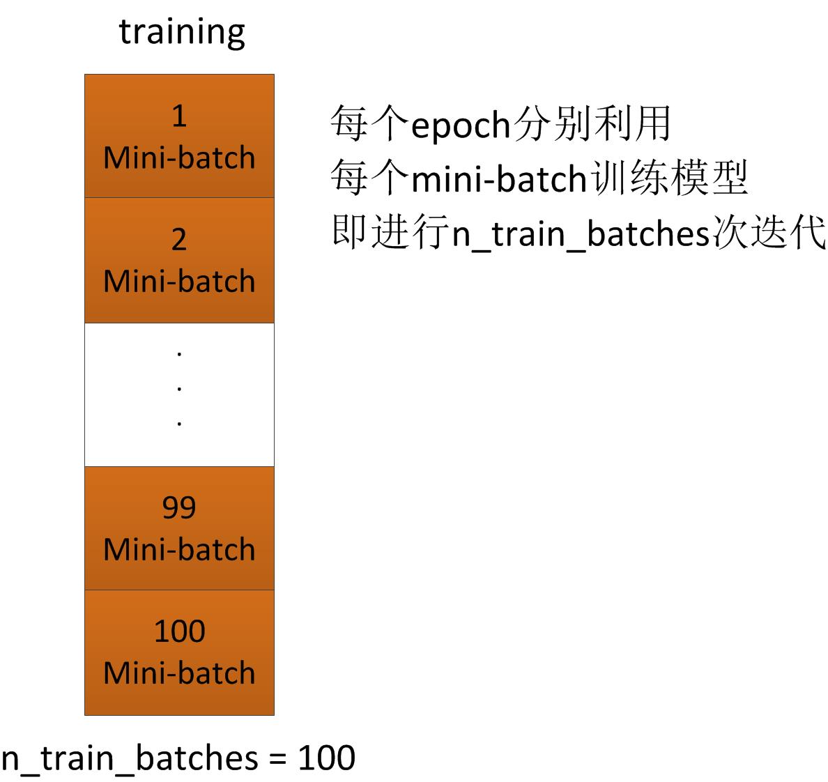
（3）Lenet-5中的training model部分

     # 开始训练模型
     print '... training'

     # 定义一些进行early-stopping的相关参数
     # look as this many examples regardless
     patience = 10000
     # wait this much longer when a new best is found
     patience_increase = 2
     # a relative improvement of this much is considered significant
     improvement_threshold = 0.995
     # go through this many minibatche before checking the network on the validation set; in this case we check every epoch
     validation_frequency = min(n_train_batches, patience / 2)

     # 训练过程中需要的其他参数
     best_validation_loss = numpy.inf
     best_iter = 0
     test_score = 0.
     start_time = timeit.default_timer()

     epoch = 0
     done_looping = False

     while (epoch < n_epochs) and (not done_looping):

         #epoch次数增加1，每轮epoch，利用所有组mini-batch进行一次模型训练
         # 每轮epoch，整体的迭代次数iter增加n_train_batches次
         epoch = epoch + 1

         # 对于整个训练集中的第minibatch_index 个mini-batch
         # minibatch_index=0,1,...,n_train_batches-1
         for minibatch_index in xrange(n_train_batches):

             # 总的iter次数（每一轮epoch，iter个数都增加n_train_batches）
             # 即每一个iter，只利用一个mini-batch进行训练
             # 而每一个epoch，利用了所有的mini-batch进行训练
             iter = (epoch - 1) * n_train_batches + minibatch_index

             # 整体的迭代次数可以被100整除时，显示一次迭代次数
             if iter % 100 == 0:
                 print 'training @ iter = ', iter

             # 利用第minibatch_index个mini-batch训练model，得到model的代价函数
             cost_ij = train_model(minibatch_index)

             # 如果整体的迭代次数满足需要进行校验的条件，则对该次iter对应的model进行校验
             if (iter + 1) % validation_frequency == 0:

                 # 计算该model在校验集上的loss函数值
                 validation_losses = [validate_model(i) for i
                                      in xrange(n_valid_batches)]
                 this_validation_loss = numpy.mean(validation_losses)
                 print('epoch %i, minibatch %i/%i, validation error %f %%' %
                       (epoch, minibatch_index + 1, n_train_batches,
                        this_validation_loss * 100.))

                 # 如果该model在校验集的loss值小于之前的值
                 if this_validation_loss < best_validation_loss:

                     # 增加patience的值，目的是为了进行更多次的iter
                     # 也就是说，如果在测试集上的性能不如之前好，证明模型开始恶化，那么，不再进行那么多次的training了
                     if this_validation_loss < best_validation_loss *  \
                        improvement_threshold:
                         patience = max(patience, iter * patience_increase)

                     # save best validation score and iteration number
                     best_validation_loss = this_validation_loss
                     best_iter = iter

                     # 利用测试集测试该模型
                     test_losses = [
                         test_model(i)
                         for i in xrange(n_test_batches)
                     ]
                     # 计算测试集的loss值
                     test_score = numpy.mean(test_losses)
                     print(('     epoch %i, minibatch %i/%i, test error of '
                            'best model %f %%') %
                           (epoch, minibatch_index + 1, n_train_batches,
                            test_score * 100.))

             if patience <= iter:
                 done_looping = True
                 break

     # 整个训练过程结束，记录training时间
     end_time = timeit.default_timer()
     print('Optimization complete.')
     print('Best validation score of %f %% obtained at iteration %i, '
           'with test performance %f %%' %
           (best_validation_loss * 100., best_iter + 1, test_score * 100.))
     print >> sys.stderr, ('The code for file ' +
                           os.path.split(__file__)[1] +
                           ' ran for %.2fm' % ((end_time - start_time) / 60.))

（4）真个convolutional_mlp的原始代码

 """This tutorial introduces the LeNet5 neural network architecture
 using Theano.  LeNet5 is a convolutional neural network, good for
 classifying images. This tutorial shows how to build the architecture,
 and comes with all the hyper-parameters you need to reproduce the
 paper's MNIST results.

 This implementation simplifies the model in the following ways:

  - LeNetConvPool doesn't implement location-specific gain and bias parameters
  - LeNetConvPool doesn't implement pooling by average, it implements pooling
    by max.
  - Digit classification is implemented with a logistic regression rather than
    an RBF network
  - LeNet5 was not fully-connected convolutions at second layer

 References:
  - Y. LeCun, L. Bottou, Y. Bengio and P. Haffner:
    Gradient-Based Learning Applied to Document
    Recognition, Proceedings of the IEEE, 86(11):2278-2324, November 1998.
    http://yann.lecun.com/exdb/publis/pdf/lecun-98.pdf

 """
 import os
 import sys
 import timeit

 import numpy

 import theano
 import theano.tensor as T
 from theano.tensor.signal import downsample
 from theano.tensor.nnet import conv

 from logistic_sgd import LogisticRegression, load_data
 from mlp import HiddenLayer

 class LeNetConvPoolLayer(object):
     """Pool Layer of a convolutional network """

     def __init__(self, rng, input, filter_shape, image_shape, poolsize=(2, 2)):
         """
         Allocate a LeNetConvPoolLayer with shared variable internal parameters.

         :type rng: numpy.random.RandomState
         :param rng: a random number generator used to initialize weights

         :type input: theano.tensor.dtensor4
         :param input: symbolic image tensor, of shape image_shape

         :type filter_shape: tuple or list of length 4
         :param filter_shape: (number of filters, num input feature maps,
                               filter height, filter width)

         :type image_shape: tuple or list of length 4
         :param image_shape: (batch size, num input feature maps,
                              image height, image width)

         :type poolsize: tuple or list of length 2
         :param poolsize: the downsampling (pooling) factor (#rows, #cols)
         """

         assert image_shape[1] == filter_shape[1]
         self.input = input

         # there are "num input feature maps * filter height * filter width"
         # inputs to each hidden unit
         fan_in = numpy.prod(filter_shape[1:])
         # each unit in the lower layer receives a gradient from:
         # "num output feature maps * filter height * filter width" /
         #   pooling size
         fan_out = (filter_shape[0] * numpy.prod(filter_shape[2:]) /
                    numpy.prod(poolsize))
         # initialize weights with random weights
         W_bound = numpy.sqrt(6. / (fan_in + fan_out))
         self.W = theano.shared(
             numpy.asarray(
                 rng.uniform(low=-W_bound, high=W_bound, size=filter_shape),
                 dtype=theano.config.floatX
             ),
             borrow=True
         )

         # the bias is a 1D tensor -- one bias per output feature map
         b_values = numpy.zeros((filter_shape[0],), dtype=theano.config.floatX)
         self.b = theano.shared(value=b_values, borrow=True)

         # convolve input feature maps with filters
         conv_out = conv.conv2d(
             input=input,
             filters=self.W,
             filter_shape=filter_shape,
             image_shape=image_shape
         )

         # downsample each feature map individually, using maxpooling
         pooled_out = downsample.max_pool_2d(
             input=conv_out,
             ds=poolsize,
             ignore_border=True
         )

         # add the bias term. Since the bias is a vector (1D array), we first
         # reshape it to a tensor of shape (1, n_filters, 1, 1). Each bias will
         # thus be broadcasted across mini-batches and feature map
         # width & height
         self.output = T.tanh(pooled_out + self.b.dimshuffle('x', 0, 'x', 'x'))

         # store parameters of this layer
         self.params = [self.W, self.b]

         # keep track of model input
         self.input = input

 def evaluate_lenet5(learning_rate=0.1, n_epochs=200,
                     dataset='mnist.pkl.gz',
                     nkerns=[20, 50], batch_size=500):
     """ Demonstrates lenet on MNIST dataset

     :type learning_rate: float
     :param learning_rate: learning rate used (factor for the stochastic
                           gradient)

     :type n_epochs: int
     :param n_epochs: maximal number of epochs to run the optimizer

     :type dataset: string
     :param dataset: path to the dataset used for training /testing (MNIST here)

     :type nkerns: list of ints
     :param nkerns: number of kernels on each layer
     """

     rng = numpy.random.RandomState(23455)

     datasets = load_data(dataset)

     train_set_x, train_set_y = datasets[0]
     valid_set_x, valid_set_y = datasets[1]
     test_set_x, test_set_y = datasets[2]

     # compute number of minibatches for training, validation and testing
     n_train_batches = train_set_x.get_value(borrow=True).shape[0]
     n_valid_batches = valid_set_x.get_value(borrow=True).shape[0]
     n_test_batches = test_set_x.get_value(borrow=True).shape[0]
     n_train_batches /= batch_size
     n_valid_batches /= batch_size
     n_test_batches /= batch_size

     # allocate symbolic variables for the data
     index = T.lscalar()  # index to a [mini]batch

     # start-snippet-1
     x = T.matrix('x')   # the data is presented as rasterized images
     y = T.ivector('y')  # the labels are presented as 1D vector of
                         # [int] labels

     ######################
     # BUILD ACTUAL MODEL #
     ######################
     print '... building the model'

     # Reshape matrix of rasterized images of shape (batch_size, 28 * 28)
     # to a 4D tensor, compatible with our LeNetConvPoolLayer
     # (28, 28) is the size of MNIST images.
     layer0_input = x.reshape((batch_size, 1, 28, 28))

     # Construct the first convolutional pooling layer:
     # filtering reduces the image size to (28-5+1 , 28-5+1) = (24, 24)
     # maxpooling reduces this further to (24/2, 24/2) = (12, 12)
     # 4D output tensor is thus of shape (batch_size, nkerns[0], 12, 12)
     layer0 = LeNetConvPoolLayer(
         rng,
         input=layer0_input,
         image_shape=(batch_size, 1, 28, 28),
         filter_shape=(nkerns[0], 1, 5, 5),
         poolsize=(2, 2)
     )

     # Construct the second convolutional pooling layer
     # filtering reduces the image size to (12-5+1, 12-5+1) = (8, 8)
     # maxpooling reduces this further to (8/2, 8/2) = (4, 4)
     # 4D output tensor is thus of shape (batch_size, nkerns[1], 4, 4)
     layer1 = LeNetConvPoolLayer(
         rng,
         input=layer0.output,
         image_shape=(batch_size, nkerns[0], 12, 12),
         filter_shape=(nkerns[1], nkerns[0], 5, 5),
         poolsize=(2, 2)
     )

     # the HiddenLayer being fully-connected, it operates on 2D matrices of
     # shape (batch_size, num_pixels) (i.e matrix of rasterized images).
     # This will generate a matrix of shape (batch_size, nkerns[1] * 4 * 4),
     # or (500, 50 * 4 * 4) = (500, 800) with the default values.
     layer2_input = layer1.output.flatten(2)

     # construct a fully-connected sigmoidal layer
     layer2 = HiddenLayer(
         rng,
         input=layer2_input,
         n_in=nkerns[1] * 4 * 4,
         n_out=500,
         activation=T.tanh
     )

     # classify the values of the fully-connected sigmoidal layer
     layer3 = LogisticRegression(input=layer2.output, n_in=500, n_out=10)

     # the cost we minimize during training is the NLL of the model
     cost = layer3.negative_log_likelihood(y)

     # create a function to compute the mistakes that are made by the model
     test_model = theano.function(
         [index],
         layer3.errors(y),
         givens={
             x: test_set_x[index * batch_size: (index + 1) * batch_size],
             y: test_set_y[index * batch_size: (index + 1) * batch_size]
         }
     )

     validate_model = theano.function(
         [index],
         layer3.errors(y),
         givens={
             x: valid_set_x[index * batch_size: (index + 1) * batch_size],
             y: valid_set_y[index * batch_size: (index + 1) * batch_size]
         }
     )

     # create a list of all model parameters to be fit by gradient descent
     params = layer3.params + layer2.params + layer1.params + layer0.params

     # create a list of gradients for all model parameters
     grads = T.grad(cost, params)

     # train_model is a function that updates the model parameters by
     # SGD Since this model has many parameters, it would be tedious to
     # manually create an update rule for each model parameter. We thus
     # create the updates list by automatically looping over all
     # (params[i], grads[i]) pairs.
     updates = [
         (param_i, param_i - learning_rate * grad_i)
         for param_i, grad_i in zip(params, grads)
     ]

     train_model = theano.function(
         [index],
         cost,
         updates=updates,
         givens={
             x: train_set_x[index * batch_size: (index + 1) * batch_size],
             y: train_set_y[index * batch_size: (index + 1) * batch_size]
         }
     )
     # end-snippet-1

     ###############
     # TRAIN MODEL #
     ###############
     print '... training'
     # early-stopping parameters
     patience = 10000  # look as this many examples regardless
     patience_increase = 2  # wait this much longer when a new best is
                            # found
     improvement_threshold = 0.995  # a relative improvement of this much is
                                    # considered significant
     validation_frequency = min(n_train_batches, patience / 2)
                                   # go through this many
                                   # minibatche before checking the network
                                   # on the validation set; in this case we
                                   # check every epoch

     best_validation_loss = numpy.inf
     best_iter = 0
     test_score = 0.
     start_time = timeit.default_timer()

     epoch = 0
     done_looping = False

     while (epoch < n_epochs) and (not done_looping):
         epoch = epoch + 1
         for minibatch_index in xrange(n_train_batches):

             iter = (epoch - 1) * n_train_batches + minibatch_index

             if iter % 100 == 0:
                 print 'training @ iter = ', iter
             cost_ij = train_model(minibatch_index)

             if (iter + 1) % validation_frequency == 0:

                 # compute zero-one loss on validation set
                 validation_losses = [validate_model(i) for i
                                      in xrange(n_valid_batches)]
                 this_validation_loss = numpy.mean(validation_losses)
                 print('epoch %i, minibatch %i/%i, validation error %f %%' %
                       (epoch, minibatch_index + 1, n_train_batches,
                        this_validation_loss * 100.))

                 # if we got the best validation score until now
                 if this_validation_loss < best_validation_loss:

                     #improve patience if loss improvement is good enough
                     if this_validation_loss < best_validation_loss *  \
                        improvement_threshold:
                         patience = max(patience, iter * patience_increase)

                     # save best validation score and iteration number
                     best_validation_loss = this_validation_loss
                     best_iter = iter

                     # test it on the test set
                     test_losses = [
                         test_model(i)
                         for i in xrange(n_test_batches)
                     ]
                     test_score = numpy.mean(test_losses)
                     print(('     epoch %i, minibatch %i/%i, test error of '
                            'best model %f %%') %
                           (epoch, minibatch_index + 1, n_train_batches,
                            test_score * 100.))

             if patience <= iter:
                 done_looping = True
                 break

     end_time = timeit.default_timer()
     print('Optimization complete.')
     print('Best validation score of %f %% obtained at iteration %i, '
           'with test performance %f %%' %
           (best_validation_loss * 100., best_iter + 1, test_score * 100.))
     print >> sys.stderr, ('The code for file ' +
                           os.path.split(__file__)[1] +
                           ' ran for %.2fm' % ((end_time - start_time) / 60.))

 if __name__ == '__main__':
     evaluate_lenet5()

 def experiment(state, channel):
     evaluate_lenet5(state.learning_rate, dataset=state.dataset)