改善深层神经网络-week1编程题（Initializaion）

Initialization

如何选择初始化方式，不同的初始化会导致不同的结果

好的初始化方式：

• 加速梯度下降的收敛(Speed up the convergence of gradient descent)

• 增加梯度下降 收敛成 一个低错误训练(和 普遍化)的几率(Increase the odds of gradient descent converging to a lower training (and generalization) error)

To get started, run the following cell to load the packages and the planar dataset you will try to classify.

import numpy as np
import matplotlib.pyplot as plt
import sklearn
import sklearn.datasets
from init_utils import sigmoid, relu, compute_loss, forward_propagation, backward_propagation
from init_utils import update_parameters, predict, load_dataset, plot_decision_boundary, predict_dec

%matplotlib inline
plt.rcParams['figure.figsize'] = (7.0, 4.0) # set default size of plots
plt.rcParams['image.interpolation'] = 'nearest'
plt.rcParams['image.cmap'] = 'gray'

# load image dataset: blue/red dots in circles
train_X, train_Y, test_X, test_Y = load_dataset()

1 - Neural Network model

你将使用一个3-layer的神经网络。有一些初始化方法你需要实现：

• Zeros initialization -- setting initialization = "zeros" in the input argument.

• Random initialization -- setting initialization = "random" in the input argument. This initializes the weights to large random values.(这个初始化权重为较大的随机值)

• He initialization -- setting initialization = "he" in the input argument. This initializes the weights to random values scaled according to a paper by He et al., 2015.

Instructions: Please quickly read over the code below, and run it. In the next part you will implement the three initialization methods that this model() calls.

def model(X, Y, learning_rate = 0.01, num_iterations = 15000, print_cost = True, initialization = "he"):
    """
    Implements a three-layer neural network: LINEAR->RELU->LINEAR->RELU->LINEAR->SIGMOID.

    Arguments:
    X -- input data, of shape (2, number of examples)
    Y -- true "label" vector (containing 0 for red dots; 1 for blue dots), of shape (1, number of examples)
    learning_rate -- learning rate for gradient descent
    num_iterations -- number of iterations to run gradient descent
    print_cost -- if True, print the cost every 1000 iterations
    initialization -- flag to choose which initialization to use ("zeros","random" or "he")

    Returns:
    parameters -- parameters learnt by the model
    """

    grads = {}
    costs = [] # to keep track of the loss
    m = X.shape[1] # number of examples
    layers_dims = [X.shape[0], 10, 5, 1]

    # Initialize parameters dictionary.
    if initialization == "zeros":
        parameters = initialize_parameters_zeros(layers_dims)
    elif initialization == "random":
        parameters = initialize_parameters_random(layers_dims)
    elif initialization == "he":
        parameters = initialize_parameters_he(layers_dims)

    # Loop (gradient descent)

    for i in range(0, num_iterations):

        # Forward propagation: LINEAR -> RELU -> LINEAR -> RELU -> LINEAR -> SIGMOID.
        a3, cache = forward_propagation(X, parameters)

        # Loss
        cost = compute_loss(a3, Y)

        # Backward propagation.
        grads = backward_propagation(X, Y, cache)

        # Update parameters.
        parameters = update_parameters(parameters, grads, learning_rate)

        # Print the loss every 1000 iterations
        if print_cost and i % 1000 == 0:
            print("Cost after iteration {}: {}".format(i, cost))
            costs.append(cost)

    # plot the loss
    plt.plot(costs)
    plt.ylabel('cost')
    plt.xlabel('iterations (per hundreds)')
    plt.title("Learning rate =" + str(learning_rate))
    plt.show()

    return parameters

2 - Zero initialization

There are two types of parameters to initialize in a neural network:

• the weight matrices \((W^{[1]}, W^{[2]}, W^{[3]}, ..., W^{[L-1]}, W^{[L]})\)
• the bias vectors \((b^{[1]}, b^{[2]}, b^{[3]}, ..., b^{[L-1]}, b^{[L]})\)

Exercise: Implement the following function to initialize all parameters to zeros. (这个不好，会"打破对称")You'll see later that this does not work well since it fails to "break symmetry", but lets try it anyway and see what happens. Use np.zeros((..,..)) with the correct shapes.

# GRADED FUNCTION: initialize_parameters_zeros 

def initialize_parameters_zeros(layers_dims):
    """
    Arguments:
    layer_dims -- python array (list) containing the size of each layer.

    Returns:
    parameters -- python dictionary containing your parameters "W1", "b1", ..., "WL", "bL":
                    W1 -- weight matrix of shape (layers_dims[1], layers_dims[0])
                    b1 -- bias vector of shape (layers_dims[1], 1)
                    ...
                    WL -- weight matrix of shape (layers_dims[L], layers_dims[L-1])
                    bL -- bias vector of shape (layers_dims[L], 1)
    """

    parameters = {}
    L = len(layers_dims)            # number of layers in the network

    for l in range(1, L):
        ### START CODE HERE ### (≈ 2 lines of code)
        parameters['W' + str(l)] = np.zeros((layers_dims[l], layers_dims[l-1]))
        parameters['b' + str(l)] = np.zeros((layers_dims[l], 1))
        ### END CODE HERE ###
    return parameters

测试:

parameters = initialize_parameters_zeros([3,2,1])
print("W1 = " + str(parameters["W1"]))
print("b1 = " + str(parameters["b1"]))
print("W2 = " + str(parameters["W2"]))
print("b2 = " + str(parameters["b2"]))

输出：

W1 = [[0. 0. 0.]
 [0. 0. 0.]]
b1 = [[0.]
 [0.]]
W2 = [[0. 0.]]
b2 = [[0.]]

Expected Output:

**W1**	[[ 0. 0. 0.] [ 0. 0. 0.]]
**b1**	[[ 0.] [ 0.]]
**W2**	[[ 0. 0.]]
**b2**	[[ 0.]]

parameters = model(train_X, train_Y, initialization = "zeros")
print ("On the train set:")
predictions_train = predict(train_X, train_Y, parameters)
print ("On the test set:")
predictions_test = predict(test_X, test_Y, parameters)

输出:

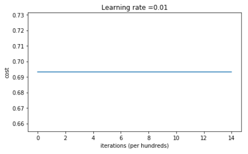
Cost after iteration 0: 0.6931471805599453

Cost after iteration 1000: 0.6931471805599453

Cost after iteration 2000: 0.6931471805599453

Cost after iteration 3000: 0.6931471805599453

Cost after iteration 4000: 0.6931471805599453

Cost after iteration 5000: 0.6931471805599453

Cost after iteration 6000: 0.6931471805599453

Cost after iteration 7000: 0.6931471805599453

Cost after iteration 8000: 0.6931471805599453

Cost after iteration 9000: 0.6931471805599453

Cost after iteration 10000: 0.6931471805599455

Cost after iteration 11000: 0.6931471805599453

Cost after iteration 12000: 0.6931471805599453

Cost after iteration 13000: 0.6931471805599453

Cost after iteration 14000: 0.6931471805599453



On the train set:

Accuracy: 0.5

On the test set:

Accuracy: 0.5

表现的非常糟糕，代价没有正真的下降，我们来看一下预测的细节 和 决策边界

print ("predictions_train = " + str(predictions_train))
print ("predictions_test = " + str(predictions_test))

predictions_train = [[0 0 0 0 0 0 0 0 0 0 0 0 0 0 0 0 0 0 0 0 0 0 0 0 0 0 0 0 0 0 0 0 0 0 0 0

0 0 0 0 0 0 0 0 0 0 0 0 0 0 0 0 0 0 0 0 0 0 0 0 0 0 0 0 0 0 0 0 0 0 0 0

0 0 0 0 0 0 0 0 0 0 0 0 0 0 0 0 0 0 0 0 0 0 0 0 0 0 0 0 0 0 0 0 0 0 0 0

0 0 0 0 0 0 0 0 0 0 0 0 0 0 0 0 0 0 0 0 0 0 0 0 0 0 0 0 0 0 0 0 0 0 0 0

0 0 0 0 0 0 0 0 0 0 0 0 0 0 0 0 0 0 0 0 0 0 0 0 0 0 0 0 0 0 0 0 0 0 0 0

0 0 0 0 0 0 0 0 0 0 0 0 0 0 0 0 0 0 0 0 0 0 0 0 0 0 0 0 0 0 0 0 0 0 0 0

0 0 0 0 0 0 0 0 0 0 0 0 0 0 0 0 0 0 0 0 0 0 0 0 0 0 0 0 0 0 0 0 0 0 0 0

0 0 0 0 0 0 0 0 0 0 0 0 0 0 0 0 0 0 0 0 0 0 0 0 0 0 0 0 0 0 0 0 0 0 0 0

0 0 0 0 0 0 0 0 0 0 0 0]]

predictions_test = [[0 0 0 0 0 0 0 0 0 0 0 0 0 0 0 0 0 0 0 0 0 0 0 0 0 0 0 0 0 0 0 0 0 0 0 0

0 0 0 0 0 0 0 0 0 0 0 0 0 0 0 0 0 0 0 0 0 0 0 0 0 0 0 0 0 0 0 0 0 0 0 0

0 0 0 0 0 0 0 0 0 0 0 0 0 0 0 0 0 0 0 0 0 0 0 0 0 0 0 0]]

plt.title("Model with Zeros initialization")
axes = plt.gca()
axes.set_xlim([-1.5,1.5])
axes.set_ylim([-1.5,1.5])
plot_decision_boundary(lambda x: predict_dec(parameters, x.T), train_X, np.squeeze(train_Y))

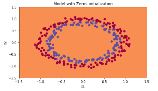
初始化0，没有能打破对称，相当于每一层神经元做着同样一件事，和 \(n^{[l]}=1\)一样

What you should remember:

• The weights \(W^{[l]}\) should be initialized randomly to break symmetry.
• It is however okay to initialize the biases \(b^{[l]}\) to zeros. Symmetry is still broken so long as \(W^{[l]}\) is initialized randomly.

3 - Random initialization

To break symmetry, lets intialize the weights randomly. Following random initialization, each neuron can then proceed to learn a different function of its inputs. In this exercise, you will see what happens if the weights are intialized randomly, but to very large values.

Exercise: Implement the following function to initialize your weights to large random values (scaled by *10) and your biases to zeros. Use np.random.randn(..,..) * 10 for weights and np.zeros((.., ..)) for biases. We are using a fixed np.random.seed(..) to make sure your "random" weights match ours, so don't worry if running several times your code gives you always the same initial values for the parameters.

# GRADED FUNCTION: initialize_parameters_random

def initialize_parameters_random(layers_dims):
    """
    Arguments:
    layer_dims -- python array (list) containing the size of each layer.

    Returns:
    parameters -- python dictionary containing your parameters "W1", "b1", ..., "WL", "bL":
                    W1 -- weight matrix of shape (layers_dims[1], layers_dims[0])
                    b1 -- bias vector of shape (layers_dims[1], 1)
                    ...
                    WL -- weight matrix of shape (layers_dims[L], layers_dims[L-1])
                    bL -- bias vector of shape (layers_dims[L], 1)
    """

    np.random.seed(3)               # This seed makes sure your "random" numbers will be the as ours
    parameters = {}
    L = len(layers_dims)            # integer representing the number of layers

    for l in range(1, L):
        ### START CODE HERE ### (≈ 2 lines of code)
        parameters['W' + str(l)] = np.random.randn(layers_dims[l], layers_dims[l-1]) * 10
        parameters['b' + str(l)] = np.zeros((layers_dims[l], 1))
        ### END CODE HERE ###

    return parameters

测试：

parameters = initialize_parameters_random([3, 2, 1])
print("W1 = " + str(parameters["W1"]))
print("b1 = " + str(parameters["b1"]))
print("W2 = " + str(parameters["W2"]))
print("b2 = " + str(parameters["b2"]))

W1 = [[ 17.88628473 4.36509851 0.96497468]

[-18.63492703 -2.77388203 -3.54758979]]

b1 = [[0.]

[0.]]

W2 = [[-0.82741481 -6.27000677]]

b2 = [[0.]]

Run the following code to train your model on 15,000 iterations using random initialization.

parameters = model(train_X, train_Y, initialization = "random")
print ("On the train set:")
predictions_train = predict(train_X, train_Y, parameters)
print ("On the test set:")
predictions_test = predict(test_X, test_Y, parameters)

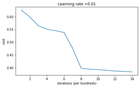
Cost after iteration 0: inf

Cost after iteration 1000: 0.6250982793959966

Cost after iteration 2000: 0.5981216596703697

Cost after iteration 3000: 0.5638417572298645

Cost after iteration 4000: 0.5501703049199763

Cost after iteration 5000: 0.5444632909664456

Cost after iteration 6000: 0.5374513807000807

Cost after iteration 7000: 0.4764042074074983

Cost after iteration 8000: 0.39781492295092263

Cost after iteration 9000: 0.3934764028765484

Cost after iteration 10000: 0.3920295461882659

Cost after iteration 11000: 0.38924598135108

Cost after iteration 12000: 0.3861547485712325

Cost after iteration 13000: 0.384984728909703

Cost after iteration 14000: 0.3827828308349524



On the train set:

Accuracy: 0.83

On the test set:

Accuracy: 0.86

If you see "inf" as the cost after the iteration 0, this is because of numerical roundoff; a more numerically sophisticated implementation would fix this. But this isn't worth worrying about for our purposes.

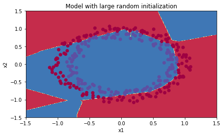
Anyway, it looks like you have broken symmetry, and this gives better results. than before. The model is no longer outputting all 0s.

print (predictions_train)
print (predictions_test)

[[1 0 1 1 0 0 1 1 1 1 1 0 1 0 0 1 0 1 1 0 0 0 1 0 1 1 1 1 1 1 0 1 1 0 0 1 1

1 1 1 1 1 1 0 1 1 1 1 0 1 0 1 1 1 1 0 0 1 1 1 1 0 1 1 0 1 0 1 1 1 1 0 0 0

0 0 1 0 1 0 1 1 1 0 0 1 1 1 1 1 1 0 0 1 1 1 0 1 1 0 1 0 1 1 0 1 1 0 1 0 1

1 0 0 1 0 0 1 1 0 1 1 1 0 1 0 0 1 0 1 1 1 1 1 1 1 0 1 1 0 0 1 1 0 0 0 1 0

1 0 1 0 1 1 1 0 0 1 1 1 1 0 1 1 0 1 0 1 1 0 1 0 1 1 1 1 0 1 1 1 1 0 1 0 1

0 1 1 1 1 0 1 1 0 1 1 0 1 1 0 1 0 1 1 1 0 1 1 1 0 1 0 1 0 0 1 0 1 1 0 1 1

0 1 1 0 1 1 1 0 1 1 1 1 0 1 0 0 1 1 0 1 1 1 0 0 0 1 1 0 1 1 1 1 0 1 1 0 1

1 1 0 0 1 0 0 0 1 0 0 0 1 1 1 1 0 0 0 0 1 1 1 1 0 0 1 1 1 1 1 1 1 0 0 0 1

1 1 1 0]]

[[1 1 1 1 0 1 0 1 1 0 1 1 1 0 0 0 0 1 0 1 0 0 1 0 1 0 1 1 1 1 1 0 0 0 0 1 0

1 1 0 0 1 1 1 1 1 0 1 1 1 0 1 0 1 1 0 1 0 1 0 1 1 1 1 1 1 1 1 1 0 1 0 1 1

1 1 1 0 1 0 0 1 0 0 0 1 1 0 1 1 0 0 0 1 1 0 1 1 0 0]]

plt.title("Model with large random initialization")
axes = plt.gca()
axes.set_xlim([-1.5,1.5])
axes.set_ylim([-1.5,1.5])
plot_decision_boundary(lambda x: predict_dec(parameters, x.T), train_X, np.squeeze(train_Y))

Observations:

• The cost starts very high. This is because with large random-valued weights, the last activation (sigmoid) outputs results that are very close to 0 or 1 for some examples, and when it gets that example wrong it incurs a very high loss for that example. Indeed, when \(\log(a^{[3]}) = \log(0)\), the loss goes to infinity.
• Poor initialization can lead to vanishing/exploding gradients(梯度消失/梯度爆炸), which also slows down the optimization algorithm.(减缓了优化算法)
• If you train this network longer you will see better results, but initializing with overly large random numbers slows down the optimization.(用过大的随机数初始化 减缓了 优化)

In summary:

• Initializing weights to very large random values does not work well. (用过大的随机数初始化工作的不是很好)
• Hopefully intializing with small random values does better. The important question is: how small should be these random values be? Lets find out in the next part! (找到，比较小的数 随机初始化)

4 - He initialization(可以解决梯度爆炸/梯度消失)

Finally, try "He Initialization"; this is named for the first author of He et al., 2015. (If you have heard of "Xavier initialization", this is similar except Xavier initialization uses a scaling factor for the weights \(W^{[l]}\) of sqrt(1./layers_dims[l-1]) where He initialization would use sqrt(2./layers_dims[l-1]).)

Exercise: Implement the following function to initialize your parameters with He initialization.

Hint: This function is similar to the previous initialize_parameters_random(...). The only difference is that instead of multiplying np.random.randn(..,..) by 10, you will multiply it by \(\sqrt{\frac{2}{\text{dimension of the previous layer}}}\), which is what He initialization recommends for layers with a ReLU activation. (每个W不是*10, 而是 * \(\sqrt{\frac{2.}{layerdims[l-1]}}\)

# GRADED FUNCTION: initialize_parameters_he

def initialize_parameters_he(layers_dims):
    """
    Arguments:
    layer_dims -- python array (list) containing the size of each layer.

    Returns:
    parameters -- python dictionary containing your parameters "W1", "b1", ..., "WL", "bL":
                    W1 -- weight matrix of shape (layers_dims[1], layers_dims[0])
                    b1 -- bias vector of shape (layers_dims[1], 1)
                    ...
                    WL -- weight matrix of shape (layers_dims[L], layers_dims[L-1])
                    bL -- bias vector of shape (layers_dims[L], 1)
    """

    np.random.seed(3)
    parameters = {}
    L = len(layers_dims) - 1 # integer representing the number of layers

    for l in range(1, L + 1):
        ### START CODE HERE ### (≈ 2 lines of code)
        parameters['W' + str(l)] = np.random.randn(layers_dims[l], layers_dims[l-1]) * (np.sqrt(2. / layers_dims[l-1]))
        parameters['b' + str(l)] = np.zeros((layers_dims[l], 1))
        ### END CODE HERE ###

    return parameters

测试：

parameters = initialize_parameters_he([2, 4, 1])
print("W1 = " + str(parameters["W1"]))
print("b1 = " + str(parameters["b1"]))
print("W2 = " + str(parameters["W2"]))
print("b2 = " + str(parameters["b2"]))

W1 = [[ 1.78862847 0.43650985]

[ 0.09649747 -1.8634927 ]

[-0.2773882 -0.35475898]

[-0.08274148 -0.62700068]]

b1 = [[0.]

[0.]

[0.]

[0.]]

W2 = [[-0.03098412 -0.33744411 -0.92904268 0.62552248]]

b2 = [[0.]]

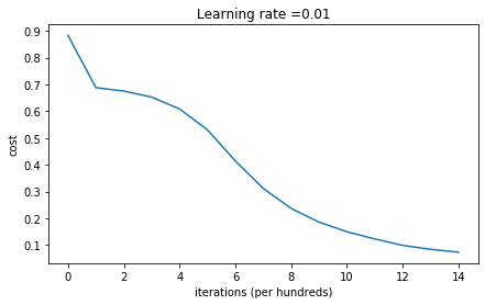
Run the following code to train your model on 15,000 iterations using He initialization.

parameters = model(train_X, train_Y, initialization = "he")
print ("On the train set:")
predictions_train = predict(train_X, train_Y, parameters)
print ("On the test set:")
predictions_test = predict(test_X, test_Y, parameters)

On the train set:

Accuracy: 0.9933333333333333

On the test set:

Accuracy: 0.96

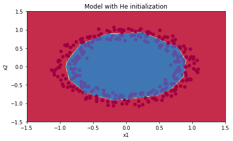
plt.title("Model with He initialization")
axes = plt.gca()
axes.set_xlim([-1.5,1.5])
axes.set_ylim([-1.5,1.5])
plot_decision_boundary(lambda x: predict_dec(parameters, x.T), train_X, np.squeeze(train_Y))

Observations:

• The model with He initialization separates the blue and the red dots very well in a small number of iterations.(工作的很好)

5 - Conclusions

You have seen three different types of initializations. For the same number of iterations and same hyperparameters the comparison is:

**Model**	**Train accuracy**	**Problem/Comment**
3-layer NN with zeros initialization	50%	fails to break symmetry
3-layer NN with large random initialization	83%	too large weights
3-layer NN with He initialization	99%	recommended method

What you should remember from this notebook:

• 不同初始化导致不同的结果
• Random initialization 能够打破对称，可以确保不同的隐藏层直接学习不同的东西
• 不要用太大的数，初始化
• He initialization works well for networks with ReLU activations.