布匹瑕疵检测数据集EDA分析

分析数据集中 train 集的每个类别的 bboxes 数量分布情况。因为训练集分了两个：train1，train2。先根据两个数据集的 anno_train.json 文件分析类别分布。数据集：布匹瑕疵检测数据集-阿里云天池 (aliyun.com)

数据集	bbox数量	缺陷图片数量	正常图片数量
train1	7728	4774	2538
train2	1795	1139	1125
总共	9523	5823	3663

EDA.py

import json
import os

import matplotlib.pyplot as plt
import seaborn as sns

#########################################
# 定义文件路径，修改成自己的anno文件路径
EDA_dir = './EDA/'
if not os.path.exists(EDA_dir):
    # shutil.rmtree(EDA_dir)
    os.makedirs(EDA_dir)

root_path = os.getcwd()
train1_json_filepath = os.path.join(root_path, "smartdiagnosisofclothflaw_round1train1_datasets",
                          "guangdong1_round1_train1_20190818", "Annotations",'anno_train.json')

train2_json_filepath = os.path.join(root_path, "smartdiagnosisofclothflaw_round1train2_datasets",
                          "guangdong1_round1_train2_20190828", "Annotations",'anno_train.json')

#########################################
# 准备数据
data1 = json.load(open(train1_json_filepath, 'r'))
data2 = json.load(open(train2_json_filepath, 'r'))

category_all = []
category_dis = {}

for i in data1:
    category_all.append(i["defect_name"])
    if i["defect_name"] not in category_dis:
        category_dis[i["defect_name"]] = 1
    else:
        category_dis[i["defect_name"]] += 1

for i in data2:
    category_all.append(i["defect_name"])
    if i["defect_name"] not in category_dis:
        category_dis[i["defect_name"]] = 1
    else:
        category_dis[i["defect_name"]] += 1

#########################################
# 配置绘图的参数
sns.set_style("whitegrid")
plt.figure(figsize=(15, 9))  # 图片的宽和高，单位为inch

# 绘制第一个子图：类别分布情况
plt.xlabel('class', fontsize=14)  # x轴名称
plt.ylabel('counts', fontsize=14)  # y轴名称
plt.xticks(rotation=90)  # x轴标签竖着显示
plt.title('Train category distribution')  # 标题
category_num = [category_dis[key] for key in category_dis]  # 制作一个y轴每个条高度列表
for x, y in enumerate(category_num):
    plt.text(x, y + 10, '%s' % y, ha='center', fontsize=10)  # x轴偏移量，y轴偏移量，数值，居中，字体大小。
ax = sns.countplot(x=category_all, palette="PuBu_r")  # 绘制直方图，palette调色板，蓝色由浅到深渐变。
# palette样式：https://blog.csdn.net/panlb1990/article/details/103851983

plt.savefig(EDA_dir + 'category_distribution.png', dpi=500)
plt.show()

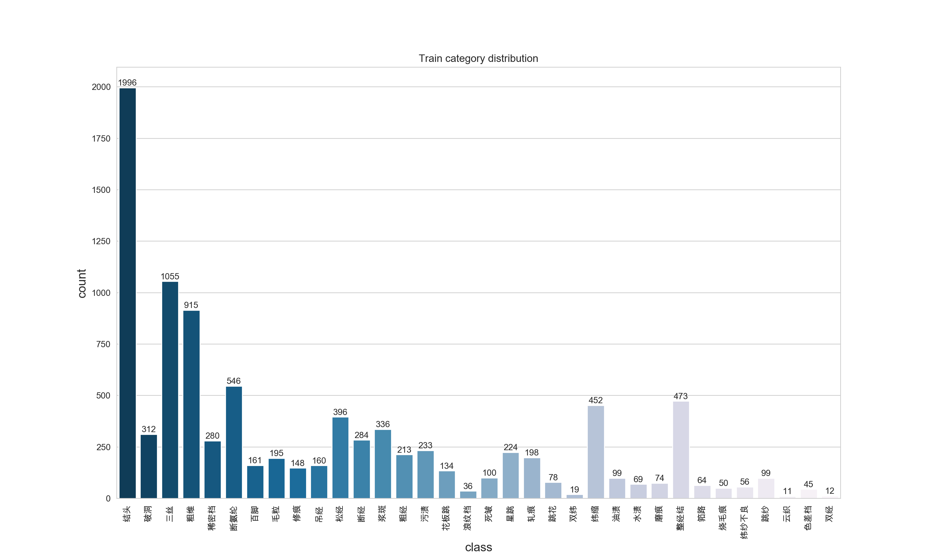
可视化结果展示：

如果你的可视化结果，matplotlib和seaborn不能显示中文，参考这里：解决python中matplotlib与seaborn画图时中文乱码的根本问题 ，亲测有用。

通过可视化结果，我们可以看出数据集中类别极不平衡，最高的1996，最低的11。接下来我们继续分析一下每个类别的宽高分布情况，以及bbox的宽高比分布情况。

EDA.py

import json
import os

import matplotlib.pyplot as plt
import seaborn as sns
#########################################
# 定义文件路径，修改成自己的anno文件路径
EDA_dir = './EDA/'
if not os.path.exists(EDA_dir):
    # shutil.rmtree(EDA_dir)
    os.makedirs(EDA_dir)

root_path = os.getcwd()
train1_json_filepath = os.path.join(root_path, "smartdiagnosisofclothflaw_round1train1_datasets",
                                    "guangdong1_round1_train1_20190818", "Annotations", 'anno_train.json')

train2_json_filepath = os.path.join(root_path, "smartdiagnosisofclothflaw_round1train2_datasets",
                                    "guangdong1_round1_train2_20190828", "Annotations", 'anno_train.json')

#########################################
# 准备数据
data1 = json.load(open(train1_json_filepath, 'r'))
data2 = json.load(open(train2_json_filepath, 'r'))

category_dis = {}
bboxes = {}
widths = {}
heights = {}
aspect_ratio={}

for i in data1:
    if i["defect_name"] not in category_dis:
        category_dis[i["defect_name"]] = 1
        bboxes[i["defect_name"]] = [i["bbox"], ]
    else:
        category_dis[i["defect_name"]] += 1
        bboxes[i["defect_name"]].append(i['bbox'])

for i in data2:
    if i["defect_name"] not in category_dis:
        category_dis[i["defect_name"]] = 1
        bboxes[i["defect_name"]] = [i["bbox"], ]
    else:
        category_dis[i["defect_name"]] += 1
        bboxes[i["defect_name"]].append(i['bbox'])

for i in bboxes:
    widths[i]=[]
    heights[i]=[]
    aspect_ratio[i]=[]
    for j in bboxes[i]:
        x1,y1,x2,y2=j
        widths[i].append(x2-x1)
        heights[i].append(y2-y1)
        aspect_ratio[i].append((x2-x1)/(y2-y1))

#########################################
# 配置绘图的参数
sns.set_style("whitegrid")
plt.figure(figsize=(15, 20))  # 图片的宽和高，单位为inch
plt.subplots_adjust(left=0.1,bottom=0.1,right=0.9,top=0.9,wspace=0.5,hspace=0.5)    # 调整子图间距

# 绘制bbox宽度和高度分布情况
for idx,i in enumerate(bboxes):
    plt.subplot(7,5,idx+1)
    plt.xlabel('width', fontsize=11)  # x轴名称
    plt.ylabel('height', fontsize=11)  # y轴名称
    plt.title(i, fontsize=13)  # 标题
    sns.scatterplot(widths[i],heights[i])

plt.savefig(EDA_dir + 'width_height_distribution.png', dpi=500, pad_inches=0)
plt.show()

# 绘制宽高比分布情况
plt.figure(figsize=(15, 20))  # 图片的宽和高，单位为inch
plt.subplots_adjust(left=0.1,bottom=0.1,right=0.9,top=0.9,wspace=0.5,hspace=0.5)    # 调整子图间距

for idx,i in enumerate(bboxes):
    plt.subplot(7,5,idx+1)
    plt.xlabel('aspect ratio', fontsize=11)  # x轴名称
    plt.ylabel('number', fontsize=11)  # y轴名称
    plt.title(i, fontsize=13)  # 标题
    sns.distplot(aspect_ratio[i],kde=False)

plt.savefig(EDA_dir + 'aspect_ratio_distribution.png', dpi=500, pad_inches=0)
plt.show()

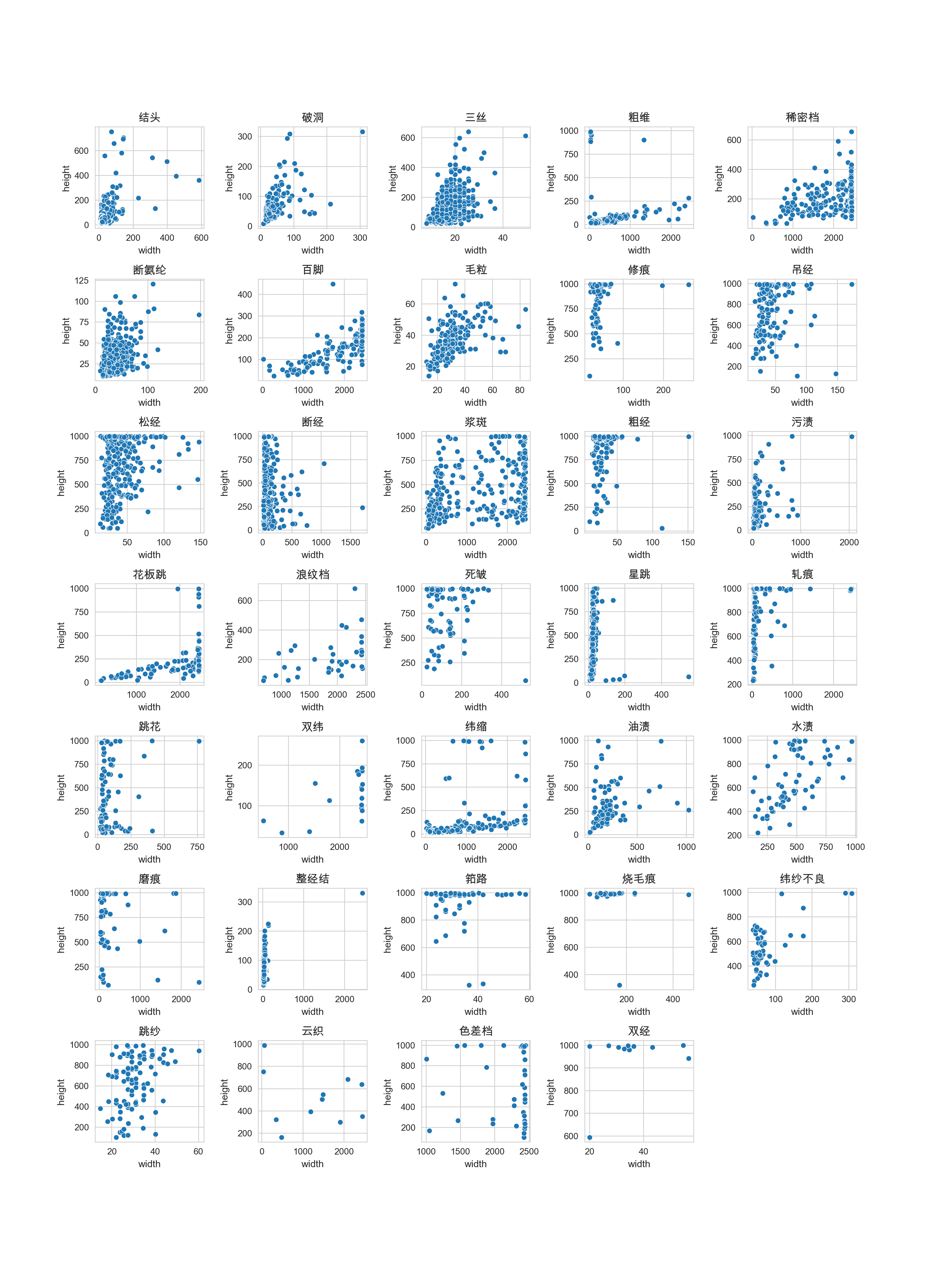
可视化结果展示：bbox宽度和高度分布情况

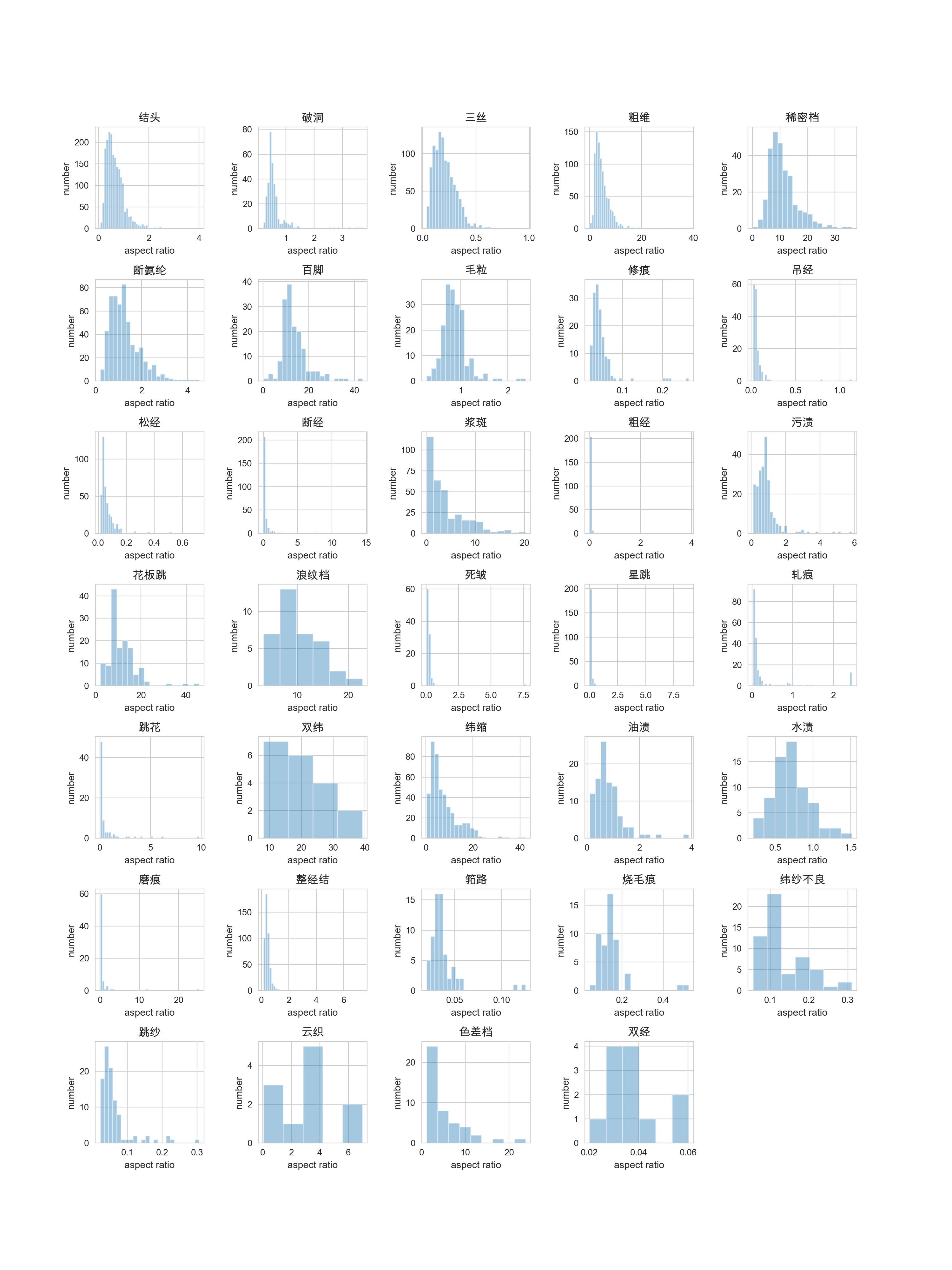
可视化结果展示：bbox宽高比的分布情况

做完所有的EDA后，可以得到以下分析：

• bbox的类别分布极不平衡。
• bbox的形状差异很大，粗维，稀密档，百脚等宽高比数值很大，部分大于10，说明bbox呈细条状。需要针对此进行修改，生成特殊比例的anchor。