[Bayes] Understanding Bayes: A Look at the Likelihood

From: https://alexanderetz.com/2015/04/15/understanding-bayes-a-look-at-the-likelihood/

Reading note.

---

Much of the discussion in psychology surrounding Bayesian inference focuses on priors. Should we embrace priors, or should we be skeptical?

When are Bayesian methods sensitive to specification of the prior, and

when do the data effectively overwhelm it?

Should we use context specific prior distributions or should we use general defaults? These are all great questions and great discussions to be having.

One thing that often gets left out of the discussion is the importance of the likelihood. The likelihood is the workhorse of Bayesian inference.

In order to understand Bayesian parameter estimation you need to understand the likelihood.

In order to understand Bayesian model comparison (Bayes factors) you need to understand the likelihood and likelihood ratios.

似然函数的重要性。

What is likelihood?

Likelihood is a funny concept. It’s not a probability, but it is proportional to a probability.

The likelihood of a hypothesis (H) given some data (D) is proportional to the probability of obtaining D given that H is true, multiplied by an arbitrary positive constant (K).

In other words, L(H|D) = K · P(D|H). Since a likelihood isn’t actually a probability it doesn’t obey various rules of probability. For example, likelihood need not sum to 1.

A critical difference between probability and likelihood is in the interpretation of what is fixed and what can vary. In the case of a conditional probability, P(D|H), the hypothesis is fixed and the data are free to vary. Likelihood, however, is the opposite. The likelihood of a hypothesis, L(H|D), conditions on the data as if they are fixed while allowing the hypotheses to vary.

The distinction is subtle, so I’ll say it again.

For conditional probability, the hypothesis is treated as a given and the data are free to vary.

For likelihood, the data are a given and the hypotheses vary.

The Likelihood Axiom

Edwards (1992, p. 30) defines the Likelihood Axiom as a natural combination of the Law of Likelihood and the Likelihood Principle.

The Law of Likelihood states that “within the framework of a statistical model, a particular set of data supports one statistical hypothesis better than another if the likelihood of the first hypothesis, on the data, exceeds the likelihood of the second hypothesis” (Emphasis original. Edwards, 1992, p. 30).

In other words, there is evidence for H1 vis-a-vis H2 if and only if the probability of the data under H1 is greater than the probability of the data under H2. That is, D is evidence for H1 over H2 if P(D|H1) >  P(D|H2). If these two probabilities are equivalent, then there is no evidence for either hypothesis over the other. Furthermore, the strength of the statistical evidence for H1 over H2 is quantified by the ratio of their likelihoods, L(H1|D)/L(H2|D) (which again is proportional to P(D|H1)/P(D|H2) up to an arbitrary constant that cancels out).

The Likelihood Principle states that the likelihood function contains all of the information relevant to the evaluation of statistical evidence. Other facets of the data that do not factor into the likelihood function are irrelevant to the evaluation of the strength of the statistical evidence (Edwards, 1992, p. 30; Royall, 1997, p. 22). They can be meaningful for planning studies or for decision analysis, but they are separate from the strength of the statistical evidence.

基础知识，貌似没啥干货。

Likelihoods are meaningless in isolation 为什么呢？

Unlike a probability, a likelihood has no real meaning per se due to the arbitrary constant. Only by comparing likelihoods do they become interpretable, because the constant in each likelihood cancels the other one out. The easiest way to explain this aspect of likelihood is to use the binomial distribution as an example.

Suppose I flip a coin 10 times and it comes up 6 heads and 4 tails. If the coin were fair, p(heads) = .5, the probability of this occurrence is defined by the binomial distribution:

where x is the number of heads obtained, n is the total number of flips, p is the probability of heads, and

Substituting in our values we get 一个似然假设，0.5

If the coin were a trick coin, so that p(heads) = .75, the probability of 6 heads in 10 tosses is: 另一个似然假设

To quantify the statistical evidence for the first hypothesis against the second, we simply divide one probability by the other. This ratio tells us everything we need to know about the support the data lends to one hypothesis vis-a-vis the other.  In the case of 6 heads in 10 tosses, the likelihood ratio (LR) for a fair coin vs our trick coin is:

这是一个似然比。

Translation: The data are 1.4 times as probable under a fair coin hypothesis than under this particular trick coin hypothesis. Notice how the first terms in each of the equations above, i.e., , are equivalent and completely cancel each other out in the likelihood ratio.

Same data. Same constant. Cancel out.

The first term in the equations above, , details our journey to obtaining 6 heads out of 10. If we change our journey (i.e., different sampling plan) then this changes the term’s value, but crucially, since it is the same term in both the numerator and denominator it always cancels itself out. In other words, the information contained in the way the data are obtained disappears from the function. Hence the irrelevance of the stopping rule to the evaluation of statistical evidence, which is something that makes bayesian and likelihood methods valuable and flexible.

If we leave out the first term in the above calculations, our numerator is L(.5) = 0.0009765625 and our denominator is L(.75) ≈ 0.0006952286. Using these values to form the likelihood ratio we get: 0.0009765625/0.0006952286 ≈ 1.4, as we should since the other terms simply cancelled out before.

Again I want to reiterate that

• the value of a single likelihood is meaningless in isolation;
• only in comparing likelihoods do we find meaning.

废话，没有似然间的比较，如何找出最大（最优的）似然。

Looking at likelihoods

Likelihoods may seem overly restrictive at first. We can only compare 2 simple statistical hypotheses in a single likelihood ratio.

But what if we are interested in comparing many more hypotheses at once? What if we want to compare all possible hypotheses at once? 比较所有可能的似然？

In that case we can plot the likelihood function for our data, and this lets us ‘see’ the evidence in its entirety.

By plotting the entire likelihood function we compare all possible hypotheses simultaneously. The Likelihood Principle tells us that the likelihood function encompasses all statistical evidence that our data can provide, so we should always plot this function along side our reported likelihood ratios. 加入了向量x，即：所有的样本信息，当然包含了我们已知的所有，必然要重视一下嘛。

Following the wisdom of Birnbaum (1962), “the “evidential meaning” of experimental results is characterized fully by the likelihood function” (as cited in Royall, 1997, p.25). So let’s look at some examples. The R script at the end of this post can be used to reproduce these plots, or you can use it to make your own plots.

Play around with it and see how the functions change for different number of heads, total flips, and hypotheses of interest. See the instructions in the script for details.

似然方程的变化？值得一看。

Below is the likelihood function for 6 heads in 10 tosses. I’ve marked our two hypotheses from before on the likelihood curve with blue dots. Since the likelihood function is meaningful only up to an arbitrary constant, the graph is scaled by convention so that the best supported value (i.e., the maximum) corresponds to a likelihood of 1. 归一化了.

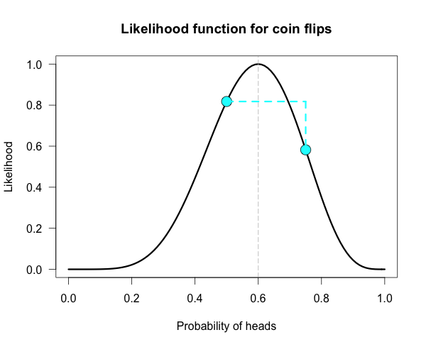
The vertical dotted line marks the hypothesis best supported by the data. The likelihood ratio of any two hypotheses is simply the ratio of their heights on this curve. We can see from the plot that the fair coin has a higher likelihood than our trick coin.

How does the curve change if instead of 6 heads out of 10 tosses, we tossed 100 times and obtained 60 heads? 数据量成比例翻倍会如何？

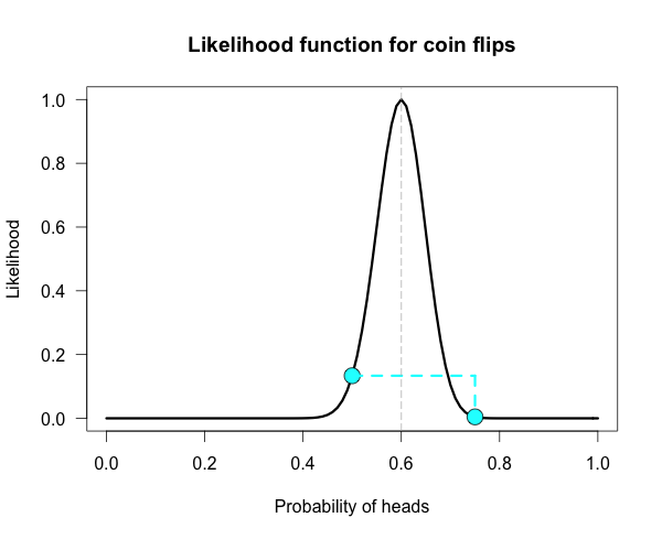
Our curve gets much narrower! 变窄了！

How did the strength of evidence change for the fair coin vs the trick coin? The new likelihood ratio is L(.5)/L(.75) ≈ 29.9. Much stronger evidence!(footnote) 数据变多，当然越多的证据支持！

However, due to the narrowing, neither of these hypothesized values are very high up on the curve anymore. It might be more informative to compare each of our hypotheses against the best supported hypothesis. This gives us two likelihood ratios:

L(.6)/L(.5) ≈ 7.5 and L(.6)/L(.75) ≈ 224.

然后要表达什么？

Here is one more curve, for when we obtain 300 heads in 500 coin flips. 数据再继续成比例变大呢？显然如下，越来越窄，但最优的，也是最可能的答案越来越值得信服。

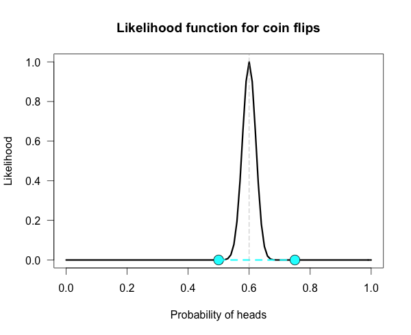
Notice that both of our hypotheses look to be very near the minimum of the graph. Yet their likelihood ratio is much stronger than before. For this data the likelihood ratio L(.5)/L(.75) is nearly 24 million! The inherent relativity of evidence is made clear here:

The fair coin was supported when compared to one particular trick coin. But this should not be interpreted as absolute evidence for the fair coin, because the likelihood ratio for the maximally supported hypothesis vs the fair coin, L(.6)/L(.5), is nearly 24 thousand!

We need to be careful not to make blanket statements about absolute support, such as claiming that the maximum is “strongly supported by the data”. Always ask, “Compared to what?”

这样看来，除非离散，否则，永远没有绝对的好点是绝对的答案。告诫大家：要相对的說。

The best supported hypothesis will be only be weakly supported vs any hypothesis just before or just after it on the x-axis. For example, L(.6)/L(.61) ≈ 1.1, which is barely any support one way or the other. It cannot be said enough that evidence for a hypothesis must be evaluated in consideration with a specific alternative.

Connecting likelihood ratios to Bayes factors

Bayes factors are simple extensions of likelihood ratios. 似然比的扩展？怎么个扩展法？

A Bayes factor is a weighted average likelihood ratio based on the prior distribution specified for the hypotheses. (When the hypotheses are simple point hypotheses, the Bayes factor is equivalent to the likelihood ratio.)

当假设检验是：simple vs simple，贝叶斯因子 就等价于 似然比。

贝叶斯因子就是：如上的后验比，除以先验比后，消去了蓝色部分，剩下的就是似然比。

The likelihood ratio is evaluated at each point of the prior distribution and weighted by the probability we assign that value.

If the prior distribution assigns the majority of its probability to values far away from the observed data, then the average likelihood for that hypothesis is lower than one that assigns probability closer to the observed data.

In other words, you get a Bayes boost if you make more accurate predictions. Bayes factors are extremely valuable, and in a future post I will tackle the hard problem of assigning priors and evaluating weighted likelihoods.

I hope you come away from this post with a greater knowledge of, and appreciation for, likelihoods. Play around with the R code and you can get a feel for how the likelihood functions change for different data and different hypotheses of interest.

总结就是：数据越多，方差越小，曲线越窄。

---

(footnote) Obtaining 60 heads in 100 tosses is equivalent to obtaining 6 heads in 10 tosses 10 separate times. To obtain this new likelihood ratio we can simply multiply our ratios together. That is, raise the first ratio to the power of 10; 1.4^10 ≈ 28.9, which is just slightly off from the correct value of 29.9 due to roundin

## Plots the likelihood function for the data obtained
## h = number of successes (heads), n = number of trials (flips),
## p1 = prob of success (head) on H1, p2 = prob of success (head) on H2
## Returns the likelihood ratio for p1 over p2. The default values are the ones used in the blog post
LR <- function(h,n,p1=.5,p2=.75){
  L1 <- dbinom(h,n,p1)/dbinom(h,n,h/n) ## Likelihood for p1, standardized vs the MLE
  L2 <- dbinom(h,n,p2)/dbinom(h,n,h/n) ## Likelihood for p2, standardized vs the MLE
  Ratio <- dbinom(h,n,p1)/dbinom(h,n,p2) ## Likelihood ratio for p1 vs p2
  curve((dbinom(h,n,x)/max(dbinom(h,n,x))), xlim = c(0,1), ylab = "Likelihood",xlab = "Probability of heads",las=1,
        main = "Likelihood function for coin flips", lwd = 3)
  points(p1, L1, cex = 2, pch = 21, bg = "cyan")
  points(p2, L2, cex = 2, pch = 21, bg = "cyan")
  lines(c(p1, p2), c(L1, L1), lwd = 3, lty = 2, col = "cyan")
  lines(c(p2, p2), c(L1, L2), lwd = 3, lty = 2, col = "cyan")
  abline(v = h/n, lty = 5, lwd = 1, col = "grey73")
  return(Ratio) ## Returns the likelihood ratio for p1 vs p2
}

LR(6, 10)