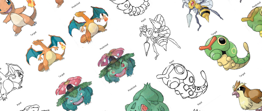
矩池云 | 教你如何使用GAN为口袋妖怪上色

在之前的Demo中，我们使用了条件GAN来生成了手写数字图像。那么除了生成数字图像以外我们还能用神经网络来干些什么呢？

在本案例中，我们用神经网络来给口袋妖怪的线框图上色。

第一步: 导入使用库

from __future__ import absolute_import, division, print_function, unicode_literals

import tensorflow as tf

tf.enable_eager_execution()

import numpy as np

import pandas as pd

import os

import time

import matplotlib.pyplot as plt

from IPython.display import clear_output

口袋妖怪上色的模型训练过程中，需要比较大的显存。为了保证我们的模型能在2070上顺利的运行，我们限制了显存的使用量为90%, 来避免显存不足的引起的错误。

config = tf.compat.v1.ConfigProto()

config.gpu_options.per_process_gpu_memory_fraction = 0.9

session = tf.compat.v1.Session(config=config)

定义需要使用到的常量。

BUFFER_SIZE = 400

BATCH_SIZE = 1

IMG_WIDTH = 256

IMG_HEIGHT = 256

PATH = 'dataset/'

OUTPUT_CHANNELS = 3

LAMBDA = 100

EPOCHS = 10

第二步: 定义需要使用的函数

图片数据加载函数，主要的作用是使用Tensorflow的io接口读入图片，并且放入tensor的对象中，方便后续使用

def load(image_file):

    image = tf.io.read_file(image_file)

    image = tf.image.decode_jpeg(image)

    w = tf.shape(image)[1]

    w = w // 2

    input_image = image[:, :w, :]

    real_image = image[:, w:, :]

    input_image = tf.cast(input_image, tf.float32)

    real_image = tf.cast(real_image, tf.float32)

    return input_image, real_image

tensor对象转成numpy对象的函数

在训练过程中，我会可视化一些训练的结果以及中间状态的图片。Tensorflow的tensor对象无法直接在matplot中直接使用，因此我们需要一个函数，将tensor转成numpy对象。

def tensor_to_array(tensor1):

    return tensor1.numpy()

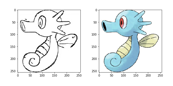
第三步: 数据可视化

我们先来看下我们的训练数据长成什么样。

我们每张数据图片分成了两个部分，左边部分是线框图，我们用来作为输入数据，右边部分是上色图，我们用来作为训练的目标图片。

我们使用上面定义的load函数来加载一张图片看下

input, real = load(PATH+'train/114.jpg')

plt.figure()

plt.imshow(tensor_to_array(input)/255.0)

plt.figure()

plt.imshow(tensor_to_array(real)/255.0)

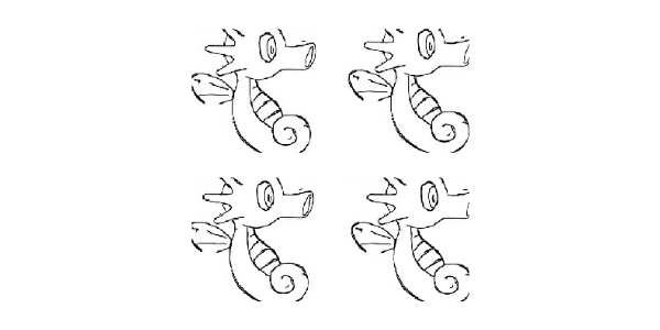
第四步: 数据增强

由于我们的训练数据不够多，我们使用数据增强来增加我们的样本。从而让小样本的数据也能达到更好的效果。

我们采取如下的数据增强方案:

图片缩放, 将输入数据的图片缩放到我们指定的图片的大小
随机裁剪
数据归一化
左右翻转

def resize(input_image, real_image, height, width):

    input_image = tf.image.resize(input_image, [height, width], method=tf.image.ResizeMethod.NEAREST_NEIGHBOR)

    real_image = tf.image.resize(real_image, [height, width], method=tf.image.ResizeMethod.NEAREST_NEIGHBOR)

    return input_image, real_image

def random_crop(input_image, real_image):

    stacked_image = tf.stack([input_image, real_image], axis=0)

    cropped_image = tf.image.random_crop(stacked_image, size=[2, IMG_HEIGHT, IMG_WIDTH, 3])

    return cropped_image[0], cropped_image[1]

def random_crop(input_image, real_image):

    stacked_image = tf.stack([input_image, real_image], axis=0)

    cropped_image = tf.image.random_crop(stacked_image, size=[2, IMG_HEIGHT, IMG_WIDTH, 3])

    return cropped_image[0], cropped_image[1]

我们将上述的增强方案做成一个函数，其中左右翻转是随机进行

@tf.function()

def random_jitter(input_image, real_image):

    input_image, real_image = resize(input_image, real_image, 286, 286)

    input_image, real_image = random_crop(input_image, real_image)

    if tf.random.uniform(()) > 0.5:

        input_image = tf.image.flip_left_right(input_image)

        real_image = tf.image.flip_left_right(real_image)

    return input_image, real_image

数据增强的效果

plt.figure(figsize=(6, 6))

for i in range(4):

    input_image, real_image = random_jitter(input, real)

    plt.subplot(2, 2, i+1)

    plt.imshow(tensor_to_array(input_image)/255.0)

    plt.axis('off')

plt.show()

第五步: 训练数据的准备

定义训练数据跟测试数据的加载函数

def load_image_train(image_file):

    input_image, real_image = load(image_file)

    input_image, real_image = random_jitter(input_image, real_image)

    input_image, real_image = normalize(input_image, real_image)

    return input_image, real_image

def load_image_test(image_file):

    input_image, real_image = load(image_file)

    input_image, real_image = resize(input_image, real_image, IMG_HEIGHT, IMG_WIDTH)

    input_image, real_image = normalize(input_image, real_image)

    return input_image, real_image

使用tensorflow的DataSet来加载训练和测试数据, 定义我们的训练数据跟测试数据集对象

train_dataset = tf.data.Dataset.list_files(PATH+'train/*.jpg')

train_dataset = train_dataset.map(load_image_train, num_parallel_calls=tf.data.experimental.AUTOTUNE)

train_dataset = train_dataset.cache().shuffle(BUFFER_SIZE)

train_dataset = train_dataset.batch(1)

test_dataset = tf.data.Dataset.list_files(PATH+'test/*.jpg')

test_dataset = test_dataset.map(load_image_test)

test_dataset = test_dataset.batch(1)

第六步: 定义模型

口袋妖怪的上色，我们使用的是GAN模型来训练, 相比上个条件GAN生成手写数字图片，这次的GAN模型的复杂读更加的高。

我们先来看下生成网络跟判别网络的整体结构

生成网络

生成网络使用了U-Net的基本框架，编码阶段的每一个Block我们使用, 卷积层->BN层->LeakyReLU的方式。解码阶段的每一个Block我们使用, 反卷积->BN层->Dropout或者ReLU。其中前三个Block我们使用Dropout, 后面的我们使用ReLU。每一个编码层的Block输出还连接了与之对应的解码层的Block. 具体可以参考U-Net的skip connection.

定义编码Block

def downsample(filters, size, apply_batchnorm=True):

    initializer = tf.random_normal_initializer(0., 0.02)

    result = tf.keras.Sequential()

    result.add(tf.keras.layers.Conv2D(filters, size, strides=2, padding='same', kernel_initializer=initializer, use_bias=False))

    if apply_batchnorm:

        result.add(tf.keras.layers.BatchNormalization())

    result.add(tf.keras.layers.LeakyReLU())

    return result

down_model = downsample(3, 4)

定义解码Block

def upsample(filters, size, apply_dropout=False):

    initializer = tf.random_normal_initializer(0., 0.02)

    result = tf.keras.Sequential()

    result.add(tf.keras.layers.Conv2DTranspose(filters, size, strides=2, padding='same', kernel_initializer=initializer, use_bias=False))

    result.add(tf.keras.layers.BatchNormalization())

    if apply_dropout:

        result.add(tf.keras.layers.Dropout(0.5))

    result.add(tf.keras.layers.ReLU())

    return result

up_model = upsample(3, 4)

定义生成网络模型

def Generator():

    down_stack = [

        downsample(64, 4, apply_batchnorm=False), # (bs, 128, 128, 64)

        downsample(128, 4), # (bs, 64, 64, 128)

        downsample(256, 4), # (bs, 32, 32, 256)

        downsample(512, 4), # (bs, 16, 16, 512)

        downsample(512, 4), # (bs, 8, 8, 512)

        downsample(512, 4), # (bs, 4, 4, 512)

        downsample(512, 4), # (bs, 2, 2, 512)

        downsample(512, 4), # (bs, 1, 1, 512)

    ]

    up_stack = [

        upsample(512, 4, apply_dropout=True), # (bs, 2, 2, 1024)

        upsample(512, 4, apply_dropout=True), # (bs, 4, 4, 1024)

        upsample(512, 4, apply_dropout=True), # (bs, 8, 8, 1024)

        upsample(512, 4), # (bs, 16, 16, 1024)

        upsample(256, 4), # (bs, 32, 32, 512)

        upsample(128, 4), # (bs, 64, 64, 256)

        upsample(64, 4), # (bs, 128, 128, 128)

    ]

    initializer = tf.random_normal_initializer(0., 0.02)

    last = tf.keras.layers.Conv2DTranspose(OUTPUT_CHANNELS, 4,

                                         strides=2,

                                         padding='same',

                                         kernel_initializer=initializer,

                                         activation='tanh') # (bs, 256, 256, 3)

    concat = tf.keras.layers.Concatenate()

    inputs = tf.keras.layers.Input(shape=[None,None,3])

    x = inputs

    skips = []

    for down in down_stack:

        x = down(x)

        skips.append(x)

    skips = reversed(skips[:-1])

    for up, skip in zip(up_stack, skips):

        x = up(x)

        x = concat([x, skip])

    x = last(x)

    return tf.keras.Model(inputs=inputs, outputs=x)

generator = Generator()

判别网络

判别网络我们使用PatchGAN, PatchGAN又称之为马尔可夫判别器。传统的基于CNN的分类模型有很多都是在最后引入了一个全连接层，然后将判别的结果输出。然而PatchGAN却不一样，它完全由卷积层构成，最后输出的是一个纬度为N的方阵。然后计算矩阵的均值作真或者假的输出。从直观上看，输出方阵的每一个输出，是模型对原图中的一个感受野，这个感受野对应了原图中的一块地方，也称之为Patch，因此，把这种结构的GAN称之为PatchGAN。

PatchGAN中的每一个Block是由卷积层->BN层->Leaky ReLU组成的。

在我们的这个模型中，最后一层我们的输出的纬度是(Batch Size, 30, 30, 1), 其中1表示图片的通道。

每个30x30的输出对应着原图的70x70的区域。详细的结构可以参考这篇论文。



def Discriminator():

    initializer = tf.random_normal_initializer(0., 0.02)

    inp = tf.keras.layers.Input(shape=[None, None, 3], name='input_image')

    tar = tf.keras.layers.Input(shape=[None, None, 3], name='target_image')

    # (batch size, 256, 256, channels*2)

    x = tf.keras.layers.concatenate([inp, tar])

    # (batch size, 128, 128, 64)

    down1 = downsample(64, 4, False)(x)

    # (batch size, 64, 64, 128)

    down2 = downsample(128, 4)(down1)

    # (batch size, 32, 32, 256)

    down3 = downsample(256, 4)(down2)

    # (batch size, 34, 34, 256)

    zero_pad1 = tf.keras.layers.ZeroPadding2D()(down3)

    # (batch size, 31, 31, 512)

    conv = tf.keras.layers.Conv2D(512, 4, strides=1, kernel_initializer=initializer, use_bias=False)(zero_pad1) 

    batchnorm1 = tf.keras.layers.BatchNormalization()(conv)

    leaky_relu = tf.keras.layers.LeakyReLU()(batchnorm1)

    # (batch size, 33, 33, 512)

    zero_pad2 = tf.keras.layers.ZeroPadding2D()(leaky_relu)

    # (batch size, 30, 30, 1)

    last = tf.keras.layers.Conv2D(1, 4, strides=1, kernel_initializer=initializer)(zero_pad2)

    return tf.keras.Model(inputs=[inp, tar], outputs=last)

discriminator = Discriminator()

第七步: 定义损失函数和优化器

**

**

loss_object = tf.keras.losses.BinaryCrossentropy(from_logits=True)



def discriminator_loss(disc_real_output, disc_generated_output):

    real_loss = loss_object(tf.ones_like(disc_real_output), disc_real_output)

    generated_loss = loss_object(tf.zeros_like(disc_generated_output), disc_generated_output)

    total_disc_loss = real_loss + generated_loss

    return total_disc_loss

def generator_loss(disc_generated_output, gen_output, target):

    gan_loss = loss_object(tf.ones_like(disc_generated_output), disc_generated_output)

    l1_loss = tf.reduce_mean(tf.abs(target - gen_output))

    total_gen_loss = gan_loss + (LAMBDA * l1_loss)

    return total_gen_loss

generator_optimizer = tf.keras.optimizers.Adam(2e-4, beta_1=0.5)

discriminator_optimizer = tf.keras.optimizers.Adam(2e-4, beta_1=0.5)

第八步: 定义CheckPoint函数

由于我们的训练时间较长，因此我们会保存中间的训练状态，方便后续加载继续训练

checkpoint = tf.train.Checkpoint(generator_optimizer=generator_optimizer,

                                 discriminator_optimizer=discriminator_optimizer,

                                 generator=generator,

                                 discriminator=discriminator)

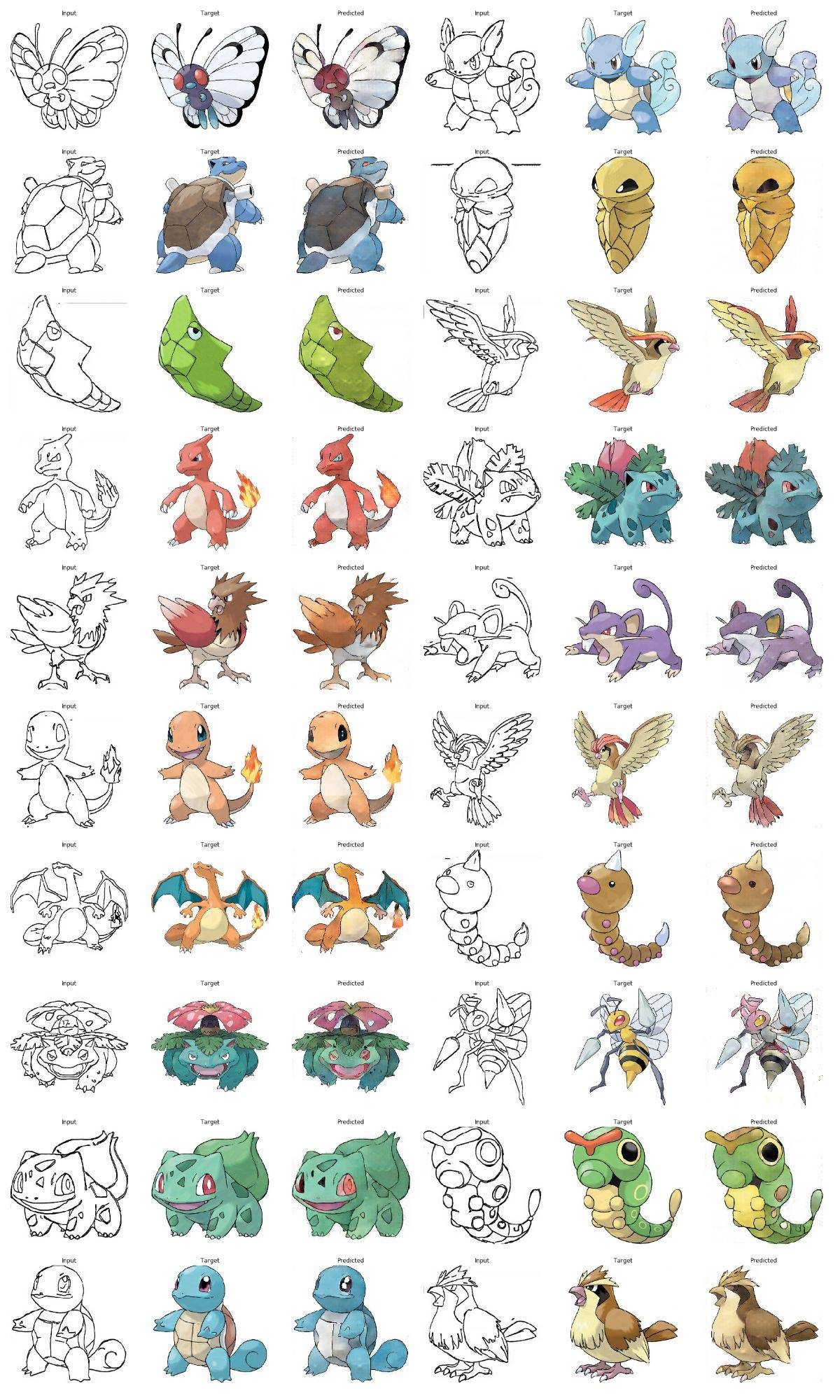
如果我们保存了之前的训练的结果，我们加载保存的数据。然后我们应用上次保存的模型来输出下我们的测试数据。

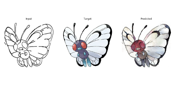
def generate_images(model, test_input, tar):

    prediction = model(test_input, training=True)

    plt.figure(figsize=(15,15))

    display_list = [test_input[0], tar[0], prediction[0]]

    title = ['Input', 'Target', 'Predicted']

    for i in range(3):

        plt.subplot(1, 3, i+1)

        plt.title(title[i])

        plt.imshow(tensor_to_array(display_list[i]) * 0.5 + 0.5)

        plt.axis('off')

    plt.show()

ckpt_manager = tf.train.CheckpointManager(checkpoint, "./", max_to_keep=2)

if ckpt_manager.latest_checkpoint:

    checkpoint.restore(ckpt_manager.latest_checkpoint)

for inp, tar in test_dataset.take(20):

    generate_images(generator, inp, tar)

第九步: 训练

在训练中，我们输出第一张图片来查看每个epoch给我们的预测结果带来的变化。让大家感受到其中的乐趣

每20个epoch我们保存一次状态

@tf.function

def train_step(input_image, target):

    with tf.GradientTape() as gen_tape, tf.GradientTape() as disc_tape:

        gen_output = generator(input_image, training=True)

        disc_real_output = discriminator([input_image, target], training=True)

        disc_generated_output = discriminator([input_image, gen_output], training=True)

        gen_loss = generator_loss(disc_generated_output, gen_output, target)

        disc_loss = discriminator_loss(disc_real_output, disc_generated_output)

    generator_gradients = gen_tape.gradient(gen_loss,

                                          generator.trainable_variables)

    discriminator_gradients = disc_tape.gradient(disc_loss,

                                               discriminator.trainable_variables)

    generator_optimizer.apply_gradients(zip(generator_gradients,

                                          generator.trainable_variables))

    discriminator_optimizer.apply_gradients(zip(discriminator_gradients,

                                              discriminator.trainable_variables))

def fit(train_ds, epochs, test_ds):

    for epoch in range(epochs):

        start = time.time()

        for input_image, target in train_ds:

            train_step(input_image, target)

        clear_output(wait=True)

        for example_input, example_target in test_ds.take(1):

            generate_images(generator, example_input, example_target)

        if (epoch + 1) % 20 == 0:

            ckpt_save_path = ckpt_manager.save()

            print ('保存第{}个epoch到{}\n'.format(epoch+1, ckpt_save_path))

        print ('训练第{}个epoch所用的时间为{:.2f}秒\n'.format(epoch + 1, time.time()-start))

fit(train_dataset, EPOCHS, test_dataset)

训练第8个epoch所用的时间为51.33秒。

第十步: 使用测试数据上色，查看下我们的效果

for input, target in test_dataset.take(20):

    generate_images(generator, input, target)

矩池云现在已经上架 “口袋妖怪上色” 镜像；感兴趣的小伙伴可以通过矩池云官网“Jupyter 教程 Demo” 镜像中尝试使用。