机器学习作业（一）线性回归——Matlab实现

题目太长啦！文档下载【传送门】

第1题

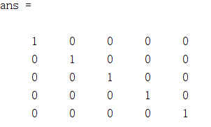
简述：设计一个5*5的单位矩阵。

function A = warmUpExercise()
A = [];
A = eye(5);
end

运行结果：

第2题

简述：实现单变量线性回归。

第1步：加载数据文件；

data = load('ex1data1.txt');
X = data(:, 1); y = data(:, 2);
m = length(y); % number of training examples
% Plot Data
% Note: You have to complete the code in plotData.m
plotData(X, y);

第2步：plotData函数实现训练样本的可视化；

function plotData(x, y)
figure;
plot(x,y,'rx','MarkerSize',10);
ylabel('Profit in $10,000s');
xlabel('Population of City in 10,000s');
end　

第3步：使用梯度下降函数计算局部最优解，并显示线性回归；

X = [ones(m, 1), data(:,1)]; % Add a column of ones to x
theta = zeros(2, 1); % initialize fitting parameters
% Some gradient descent settings
iterations = 1500;
alpha = 0.01;
% run gradient descent
theta = gradientDescent(X, y, theta, alpha, iterations);
% print theta to screen
fprintf('Theta found by gradient descent:\n');
fprintf('%f\n', theta);
% Plot the linear fit
hold on; % keep previous plot visible
plot(X(:,2), X*theta, '-')
legend('Training data', 'Linear regression')
hold off % don't overlay any more plots on this figure　　

第4步：实现梯度下降gradientDescent函数；

function [theta, J_history] = gradientDescent(X, y, theta, alpha, num_iters)

% Initialize some useful values
m = length(y); % number of training examples
J_history = zeros(num_iters, 1);

for iter = 1:num_iters
    theta = theta - alpha/length(y)*(X'*(X*theta-y))；
    % Save the cost J in every iteration
    J_history(iter) = computeCost(X, y, theta);
end

end

第5步：实现代价计算computeCost函数；

function J = computeCost(X, y, theta)
m = length(y); % number of training examples
J = 1/(2*m)*sum((X*theta-y).^2)；
end

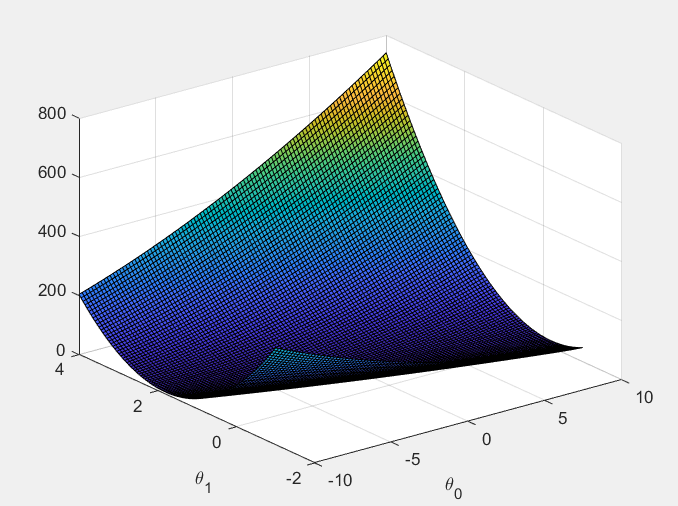
第6步：实现三维图、轮廓图的显示。

% Grid over which we will calculate J
theta0_vals = linspace(-10, 10, 100);
theta1_vals = linspace(-1, 4, 100);

% initialize J_vals to a matrix of 0's
J_vals = zeros(length(theta0_vals), length(theta1_vals));

% Fill out J_vals
for i = 1:length(theta0_vals)
    for j = 1:length(theta1_vals)
	  t = [theta0_vals(i); theta1_vals(j)];
	  J_vals(i,j) = computeCost(X, y, t);
    end
end

% Because of the way meshgrids work in the surf command, we need to
% transpose J_vals before calling surf, or else the axes will be flipped
J_vals = J_vals';
% Surface plot
figure;
surf(theta0_vals, theta1_vals, J_vals)；
xlabel('\theta_0'); ylabel('\theta_1');

% Contour plot
figure;
% Plot J_vals as 15 contours spaced logarithmically between 0.01 and 100
contour(theta0_vals, theta1_vals, J_vals, logspace(-2, 3, 20))
xlabel('\theta_0'); ylabel('\theta_1');
hold on;
plot(theta(1), theta(2), 'rx', 'MarkerSize', 10, 'LineWidth', 2);

运行结果：

第3题

简述：实现多元线性回归。

第1步：加载数据文件；

data = load('ex1data2.txt');
X = data(:, 1:2);
y = data(:, 3);
m = length(y);
[X mu sigma] = featureNormalize(X);
% Add intercept term to X
X = [ones(m, 1) X];

第2步：均值归一化featureNormalize函数实现；

function [X_norm, mu, sigma] = featureNormalize(X)

X_norm = X;
mu = zeros(1, size(X, 2));
sigma = zeros(1, size(X, 2));
mu = mean(X,1)；
sigma = std(X,0,1)；
X_norm = (X_norm-mu)./sigma；

end

第3步：使用梯度下降函数计算局部最优解，并显示线性回归；

% Choose some alpha value
alpha = 0.05;
num_iters = 100;

% Init Theta and Run Gradient Descent
theta = zeros(3, 1);
[theta, J_history] = gradientDescentMulti(X, y, theta, alpha, num_iters);

% Plot the convergence graph
figure;
plot(1:numel(J_history), J_history, '-b', 'LineWidth', 2);
xlabel('Number of iterations');
ylabel('Cost J');

第4步：实现梯度下降gradientDescentMulti函数；

function [theta, J_history] = gradientDescentMulti(X, y, theta, alpha, num_iters)

m = length(y); % number of training examples
J_history = zeros(num_iters, 1);

for iter = 1:num_iters
    theta = theta - alpha/m*(X'*(X*theta-y));
    % Save the cost J in every iteration
    J_history(iter) = computeCostMulti(X, y, theta);
end

end

第5步：实现代价计算computeCostMulti函数；

function J = computeCostMulti(X, y, theta)
m = length(y); % number of training examples
J = 1/(2*m)*sum((X*theta-y).^2)；%J=(X*theta-y)'*(X*theta-y)/(2*m);
end

运行结果：

第6步：使用上述结果对“the price of a 1650 sq-ft, 3 br house”进行预测；

X1 = [1,1650,3];
X1(2:3) = (X1(2:3)-mu)./sigma;
price = X1*theta;

预测结果：　

第7步：使用正规方程法求解；

%%Load Data
data = csvread('ex1data2.txt');
X = data(:, 1:2);
y = data(:, 3);
m = length(y);

% Add intercept term to X
X = [ones(m, 1) X];

% Calculate the parameters from the normal equation
theta = normalEqn(X, y);

第8步：实现normalEqn函数；

function [theta] = normalEqn(X, y)
theta = zeros(size(X, 2), 1);
theta = (X'*X)^(-1)*X'*y；
end

第9步：使用上述结果对“the price of a 1650 sq-ft, 3 br house”再次进行预测；

price = [1,1650,3]*theta；

预测结果：（与梯度下降法结果很接近）